1. Introduction
Sequence Modeling:
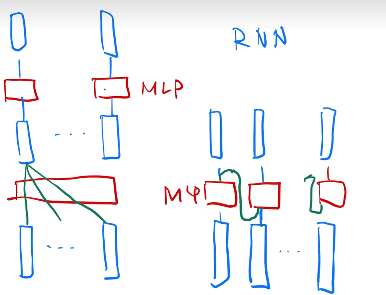
Recurrent language modelsExtension of Abstract.
- Operate step-by-step, processing one token or time step at a time.
- one input + hidden state → one output + hidden state (update every time)
- e.g., RNNs, LSTMs
Encoder-decoder architectures
- Composed of two RNNs (or other models):
- one to encode input into a representation
- another to decode it into the output sequence
- one input + hidden state → … → hidden state → one output + hidden state → …
- e.g., seq2seq
Disadvantages about these two:
Recurrent models preclude parallelization, so it’s not good.
Encoder-decoder models have used attention to pass the stuff from encoder to decoder more effectively.
Attention doesn’t use recurrence and entirely relies on an attention mechanism to draw glabal dependencies between input and output.
2. Background
Reduce sequential computation:
Typically use convolutional neural networks → the number of operations grows in the distance between positions → transfomer: a constant number of operations
- at the cost of reduced effective resolution due to averaging attention-weighted positions
- we counteract this bad effect with Multi-Head Attention
Self-attention:
compute a representation of the sequence based on different positions
End-to-end memory networks:
✔ Reccurrence attention mechanism
❌ Sequence-aligned recurrence
Transformer:
The first transduction model relying entirely on self-attention to do encoder-decoder model. ( to compute representations of its input and output without using sequence-aligned RNNs or convolution)
transduction model refers to making predictions or inferences about specific instances based on the data at hand, without relying on a prior generalization across all possible examples, which is different from Inductive learning.
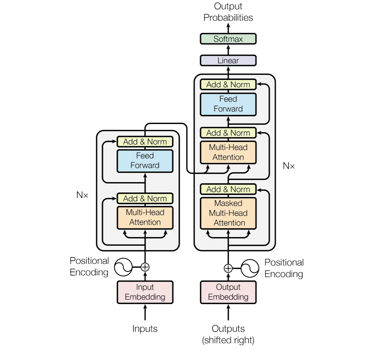
3. Model Architecture
The Transformer uses stacked self-attention and point-wise, fully connected layers for both the encoder and the decoder.
- Encoder: maps an input sequence of symbol representations x → a sequence of continuous representations z.
- Decoder: given z, generates an output sequence of symbols one element at a time. At each step, the model is auto-regressive.
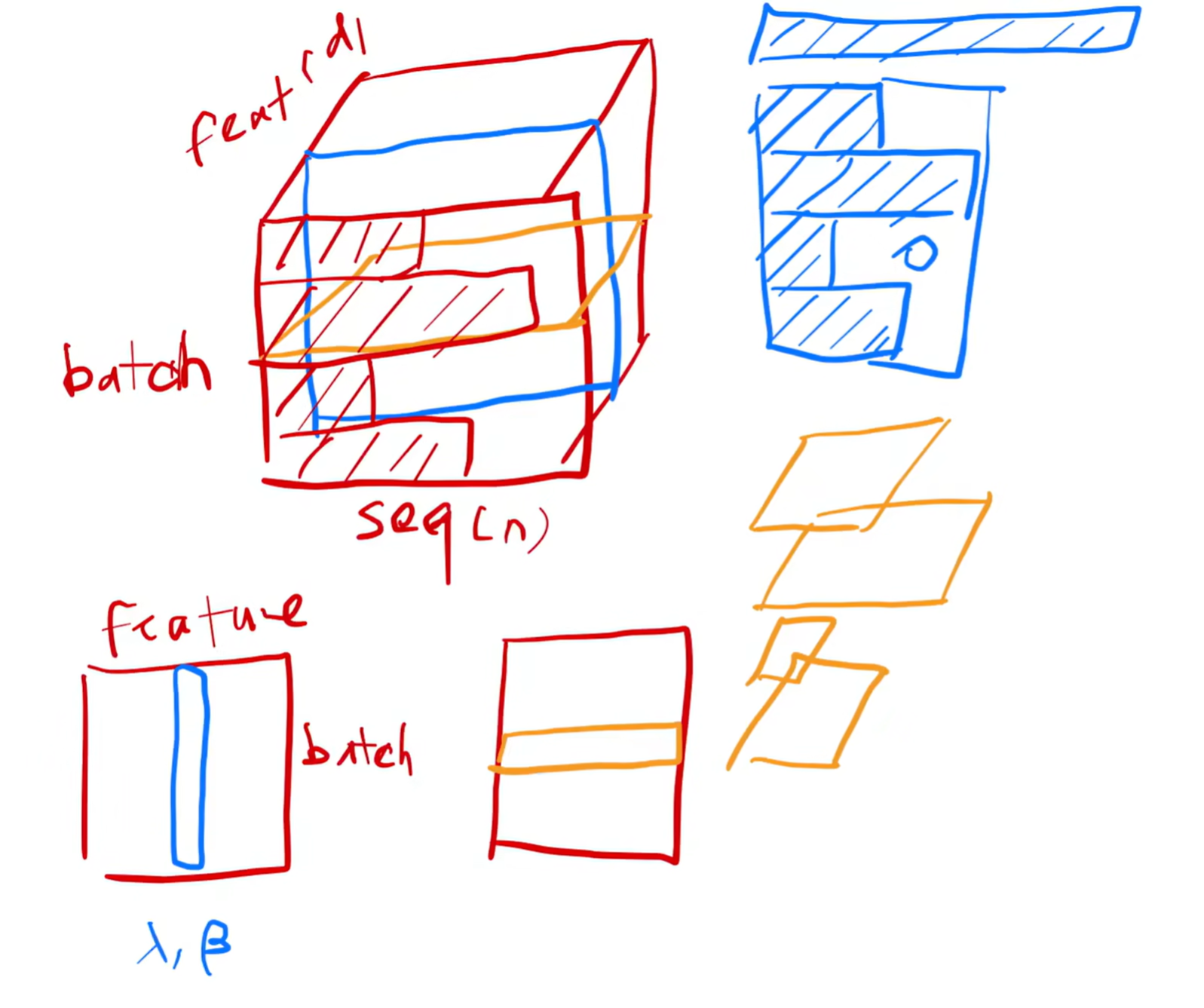
Why Using LayerNorm not BatchNorm?
LayerNorm normalizes across features of a single sample, suitable for variable-length sequences.
BatchNorm normalizes across the batch, which can be inconsistent for sequence tasks.
3.1 Encoder and Decoder Stacks
Encoder
N = 6 identical layers, each layer has two sub-layers.
- multi-head self-attention mechanism
- simple, position-wise fully connected feed-forward network
For each sub-layer, connect a layer normalization and a residual connection.
dimension of output = 512
Decoder
N = 6 identical layers, each layer has three sub-layers.
- masked multi-head attention over the output of the encoder stack
- multi-head self-attention mechanism
- simple, position-wise fully connected feed-forward network
For each sub-layer, connect a layer normalization and a residual connection.
3.2 Attention
An attention function can be described as mapping a query and a set of key-value pairs to an output where the query, keys, values, and output are all vectors.
The output is computed as a weighted sum of the values, where the weight assigned to each value is computed by a compatibility function of the query with the corresponding key.
( Given a query, output is computed by similarity between query and keys, then different keys have different weights, next combine the values based on the weights. )
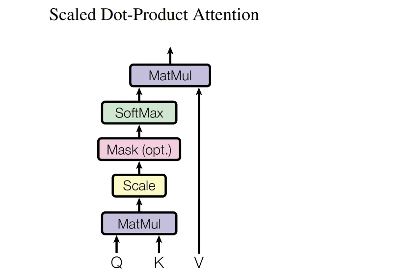
3.2.1 Scaled Dot-Product Attention
We compute the dot products of the query with all keys, divide each by length of query √, and apply a softmax function to obtain the weights on the values.
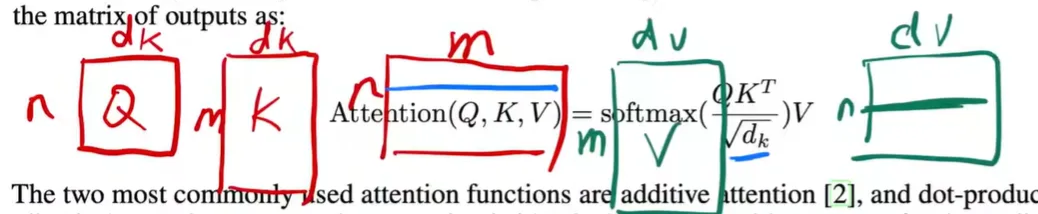
n refers to the length of a sequence, the number of the words.
dk refers to the length of the one word vector.
m refers to the number of the target words.
dv refers to the length of the one target word vector.
3.2.2 Multi-Head Attention
Linear projection, just like lots of channels.
Linearly project the queries, keys and values h times to low dimensions with different, learned linear projections.
Finally, these are concatenated (stack) and once again projected.
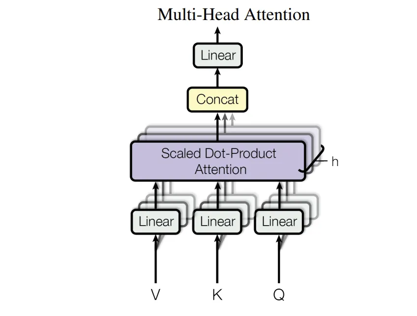
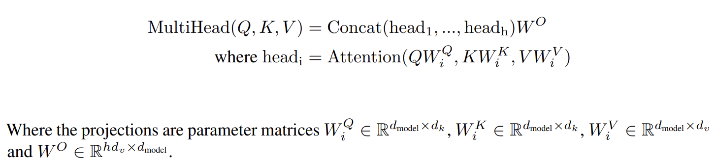
We emply h = 8 parallel attention layers, or heads.
So for each layer or head, we make their dimension to 64 to make the total computational cost is similar to single-head attention.
3.2.3 Application of Attention in our Model
The Transformer uses multi-head attention in three different ways:
- In “encoder-decoder attention” layers,
- queries → previous decoder layer
- keys and values → the output of the encoder
- In “encoder self-attention” layers,
- keys, values and queries all come from the previous layer in the encoder
- In “decoder self-attention” layers,
- keys, values and queries all come from the previous layer in the decoder
- allow each position in the decoder to attend to all positions in the decoder up to and including that position
3.3 Position-wise Feed-Forward Networks
The fully connected feed-forward network is applied to each position separately and identically.
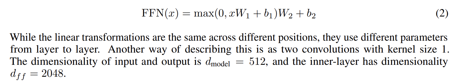
The Multi-Head Attention has already get the location information, now we need to add more expression ability by adding non-linear.
3.4 Embedding and Softmax
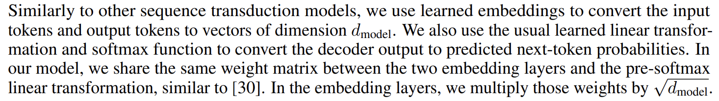
Embedding
convert the input tokens to vectors of dimension ( 512 ), then multiply those weights by
$\sqrt {d_{models}}$
Softmax
convert the decoder output to predicted next-token probabilities.
3.5 Positional Encoding
The order change, but the values don’t change. So we add the sequential information to the input.
We use sine and cosine functions of different frequencies [-1, 1]

4. Why Self-Attention
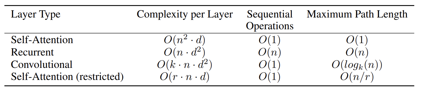
- Length of a word → d
- Number of words → n
- Self-Attention → n words ✖️ every words need to multiply with n words and for each two words do d multiplying.
- Recurrent → d-dimension vector multiply d✖️d matrix, n times
- Convolutional → k kernel_size, n words, d^2 input_channels ✖️ output_channels (Draw picture clear)
- Self-Attention (restricted) → r the number of neighbors
It seems like Self-Attention architecture has lots of advantages, but it needs more data and bigger model to train to achieve the same effect.
5. Training
5.1 Training Data and Batching
Sentences were encoded using byte-pair encoding, which has a shared source-target vocabulary of about 37000 tokens. → So we share the same weight matrix between the two embedding layers and the pre-softmax linear transformation.
5.2 Hardware and Schedule
5.3 Optimizer
5.4 Regularization
- Residual Dropout
- Label Smoothing
6. Results

$N:$ number of blocks
$d_{model}:$ the length of a token vector
$d_{ff}:$ Feed-Forward Full-Connected Layer Intermediate layer output size
$h:$ the number of heads
$d_k:$ the dimension of keys in a head
$d_v :$ the dimension of values in a head
$P_{drop}:$ dropout rate
$\epsilon_{ls}:$ Label Smoothing value, the learned label value
$train steps:$ the number of batchs