Abstract
What’s the Reference-based Super-resolution (RefSR) Network:
- Super-resolves a low-resolution (LR) image given an external high-resolution (HR) reference image
- The reference image and LR image share similar viewpoint but with significant resolution gap (8×).
Solve the problem
- Existing RefSR methods work in a cascaded way such as patch matching followed by synthesis pipeline with two independently defined objective functions
- Divide the image into many small patches (like tiny squares), each patch is compared with a reference image to find its most similar region.
- But every patch makes its decision independently. → Inter-patch misalignment
- Because of the small misalignments, the grid of patch boundaries in the final image shows. → Grid artifacts
- Old methods trained two steps separately → Inefficient training
- The challenge large-scale (8×) super-resolution problem
- the spatial resolution is increased by 8 times in each dimension (width and height).
- So the total number of pixels increases from 8×8 to 64×64.
- patch matching → warping
Structure:
- image encoders
- extract multi-scale features from both the LR and the reference images
- cross-scale warping layers
- spatially aligns the reference feature map with the LR feature map
- warping module originated from spatial transformer network (STN)
- fusion decoder
- aggregates feature maps from both domains to synthesize the HR output
| Scale | Resolution (relative) | Example size | What it focuses on |
|---|---|---|---|
| Scale 0 | ×1 (full resolution) | 512×512 | Fine details (small shifts) |
| Scale 1 | ×2 smaller | 256×256 | Medium motions |
| Scale 2 | ×4 smaller | 128×128 | Larger motions |
| Scale 3 | ×8 smaller | 64×64 | Very large motions |
| Scale 4–5 | ×16, ×32 smaller | 32×32, 16×16 | Extremely coarse view (too little detail) |
Result
Using cross-scale warping, our network is able to perform spatial alignment at pixel-level in an end-to-end fashion, which improves the existing schemes both in precision (around 2dB-4dB) and efficiency (more than 100 times faster).
- spatial alignment at pixel-level → precision and efficiency
- precision
- efficiency
1. Introduction
The two critical issues in RefSR:
- Image correspondence between the two input images
- High resolution synthesis of the LR image.
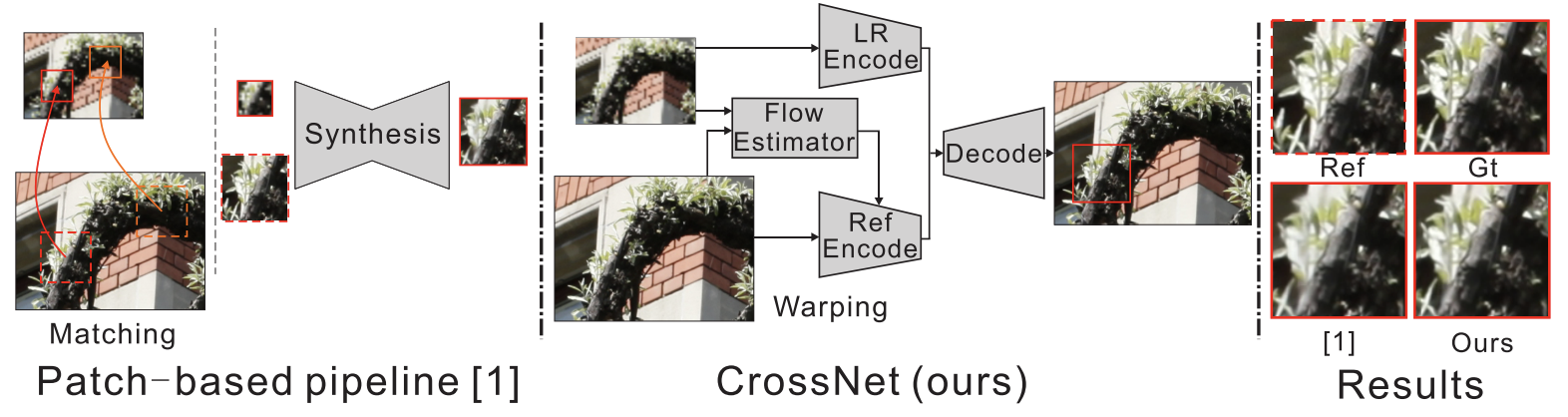
The ‘patch maching + synthesis’ pipeline → the end-to-end CrossNet → results comparisons.
Non-rigid deformation: when an object changes its shape or structure in the image (for example, bending, twisting, or changing due to different camera angles).
- Rigid = only simple shifts, rotation, or scaling.
- Non-rigid = more complex distortions — like bending, stretching, or perspective change.
Grid artifacts: visible blocky or checker-like patterns that appear because the image was reconstructed from many small, rigid square patches that don’t align smoothly.
- Grid artifacts occur when an image is reconstructed from many small square patches that don’t align perfectly at their borders.
The Laplacian is a mathematical operator that measures how much a pixel value differs from its surroundings.
In other words, it tells you where the image changes quickly — that’s usually at edges or texture details.
2. Related Work
Multi-scale deep super resolution
we employ MDSR as a sub-module for LR images feature extraction and RefSR synthesis.
- MDSR stands for Multi-scale Deep Super-Resolution Network
- Used for
- Feature extraction → understanding what’s in the LR image
- RefSR synthesis → combining LR and reference features to output the high-resolution result
Warping and synthesis
We follow such “warping and synthesis” pipeline. However, our approach is different from existing works in the following ways:
- Our approach performs multi-scale warping on feature domain
at pixel-scale- which accelerates the model convergence by allowing flow to be globally updated at higher scales.
- a novel fusion scheme is proposed for image synthesis.
concatenation,linearly combining images
3. Approach
3.1 Fully Conv Cross-scale Alignment Module
It is necessary to perform spatial alignment for reference image, since it is captured at different view points from LR image.
Cross-scale warping
We propose cross-scale warping to perform non-rigid image transformation.
Our proposed cross-scale warping operation considers a pixel-wise shift vector ( V ):
$$ I_o = warp(y_{Ref}, V) $$
which assigns a specific shift vector for each pixel location, so that it avoids the blocky and blurry artifacts.
Cross-scale flow estimator
Purpose: Predict pixel-wise flow fields to align the upsampled LR image with the HR reference.
Model: Based on FlowNetS, adapted for multi-scale correspondence.
Inputs:
- $I_{LR↑}$ : LR image upsampled by MDSR (SISR)
- $I_{REF}$ : reference image
Outputs: Multi-scale flow fields
${V^{(3)}, V^{(2)}, V^{(1)}, V^{(0)}}$ (coarse → fine).
Modification: ×4 bilinear upsampling with → two ×2 upsampling modules + skip connections + deconvolution → finer, smoother flow prediction.
Advantage:
- Captures both large and small displacements;
- Enables accurate, non-rigid alignment
- Reduces warping artifacts.
3.2 End-to-end Network Structure
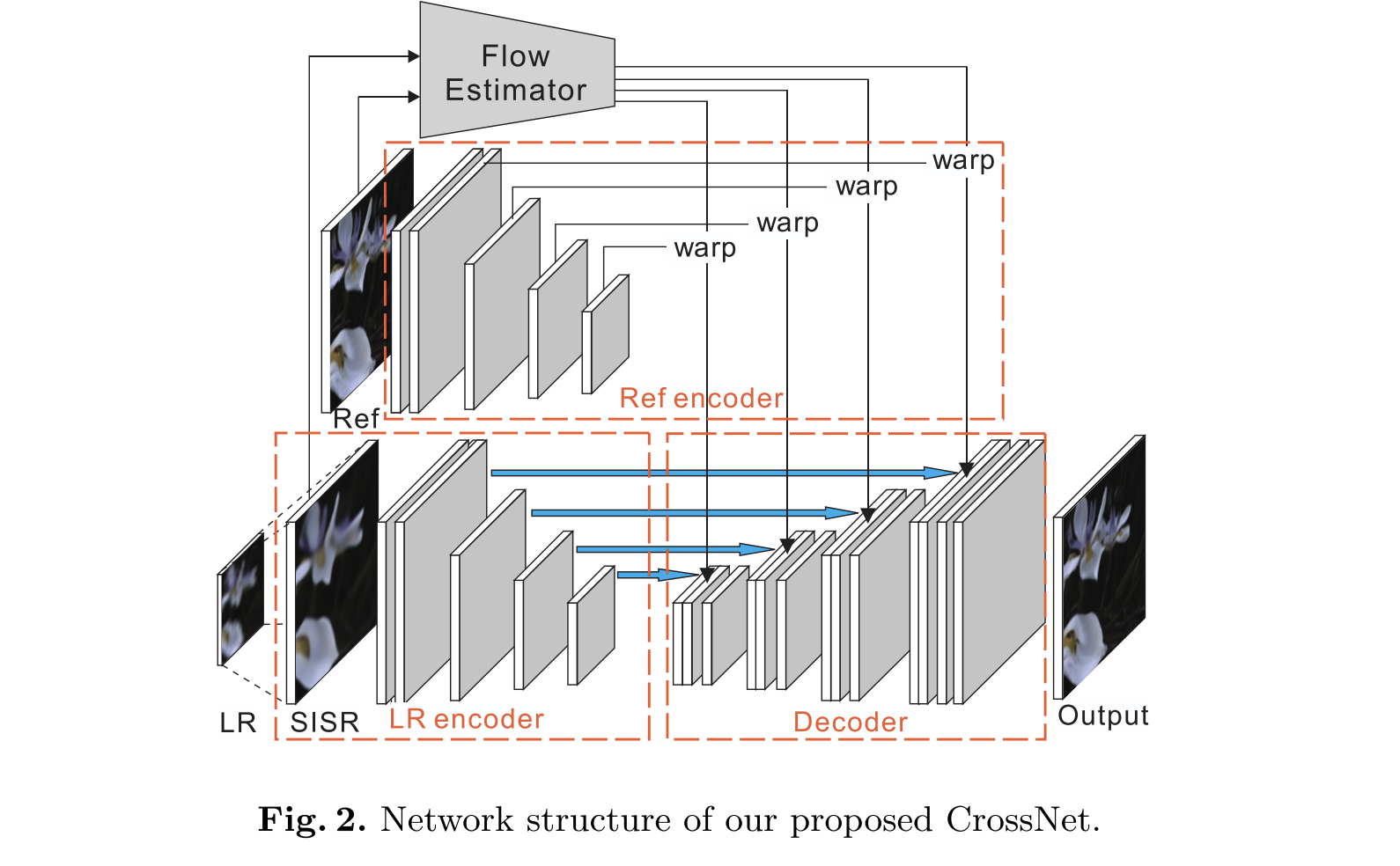
Network structure of CrossNet
LR image Encoder
Goal: Extract multi-scale feature maps from the low-resolution (LR) image for alignment and fusion.
Structure:
- Uses a Single-Image SR (SISR) upsampling to enlarge the LR image first.
- Then applies 4 convolutional layers (5×5 filters, 64 channels).
- Each layer creates a feature map at a different scale (0 → 3).
- Stride = 1 for the first layer, stride = 2 for deeper ones (downsampling by 2).
Output:
- A set of multi-scale LR feature maps.
$$ F_{LR}^{(0)}, F_{LR}^{(1)}, F_{LR}^{(2)}, F_{LR}^{(3)} $$
Activation: ReLU (σ).
Reference image encoder
Goal: Extract and align multi-scale reference features from the HR reference image.
Structure:
- Uses the same 4-scale encoder design as the LR encoder.
- Produces feature maps .
$$ {F_{REF}^{(0)}, F_{REF}^{(1)}, F_{REF}^{(2)}, F_{REF}^{(3)}} $$
- LR and reference encoders have different weights, allowing complementary feature learning.
Alignment:
- Each reference feature map $F_{REF}^{(i)}$ is warped using the cross-scale flow $V^{(i)}$.
- This generates spatially aligned reference features
$$ \hat{F}{REF}^{(i)} = warp(F_{REF}^{(i)}, V^{(i)}) $$
Decoder
- Goal: Fuse the low-resolution (LR) features and warped reference (Ref) features across multiple scales to reconstruct the super-resolved (SR) image.
- Structure Overview
- The decoder follows a U-Net–like architecture.
- It performs multi-scale fusion and up-sampling using deconvolution layers.
- Each scale combines:
- The LR feature at that scale $F_{LR}^{(i)}$,
- The warped reference feature $\hat{F}_{REF}^{(i)}$,
- The decoder feature from the next coarser scale $F_{D}^{(i+1)}$ (if available).
3.3 Loss Function
Goal: Train CrossNet to generate super-resolved (SR) outputs $I_p$ close to the ground-truth HR images $I_{HR}$.
Formula:
$$ L = \frac{1}{N} \sum_{i=1}^{N} \sum_{s} \rho(I_{HR}^{(i)}(s) - I_{p}^{(i)}(s)) $$
Penalty: Uses the Charbonnier loss
$$ \rho(x) = \sqrt{x^2 + 0.001^2} $$
A smooth, robust version of L1 loss that reduces the effect of outliers.
Variables:
- $N$: number of training samples
- $s$: pixel (spatial location)
- $i$: training sample index
4. Experiment
4.1 Dataset
- Dataset:
- The representative Flower dataset and Light Field Video (LFVideo) dataset.
- Each light field image has:
- 376 × 541 spatial samples
- 14 × 14 angular samples
- Model training:
- Each light field image has:
- 320 × 512 spatial samples
- 8 × 8 angular samples
- Each light field image has:
- Test generalization:
- Datasets:
- Stanford Light Field dataset
- Scene Light Field dataset
- Datasets:
- During testing, they apply the big input images using a sliding window approach:
- Window size: 512×512
- Stride: 256
4.2 Evaluation
- Training setup:
- Trained for 200K iterations on Flower and LFVideo datasets.
- Scale factors: ×4 and ×8 super-resolution.
- Learning rate: 1e-4 / 7e-5 → decayed to 1e-5 / 7e-6 after 150K iterations.
- Optimizer: Adam (β₁ = 0.9, β₂ = 0.999).
- Comparisons:
- Competes with RefSR methods (SS-Net, PatchMatch) and SISR methods (SRCNN, VDSR, MDSR).
- Evaluation metrics:
- PSNR, SSIM, and IFC on ×4 and ×8 scales.
- Reference images from position (0,0); LR images from (1,1) and (7,7).
- Results:
- CrossNet achieves 2–4 dB PSNR gain over previous methods.
- CrossNet consistently outperforms the resting approaches under different disparities, datasets and scales.
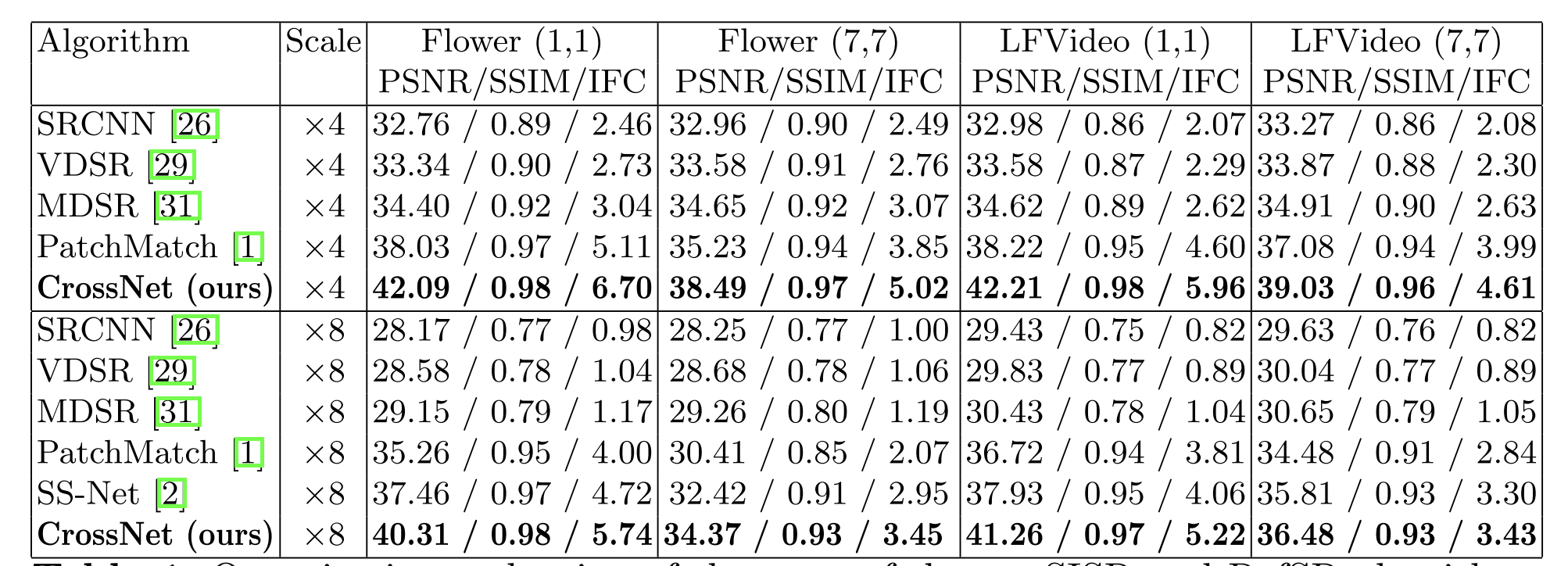
Quantitative evaluation of the sota SISR and RefSR algorithms, in terms of PSNR/SSIM/IFC for scale factors ×4 and ×8 respectively.
| Metric | Meaning |
|---|---|
| PSNR (Peak Signal-to-Noise Ratio) | Measures reconstruction accuracy (higher = clearer, less error). |
| SSIM (Structural Similarity Index) | Measures structural similarity to the ground truth (higher = more visually similar). |
| IFC (Information Fidelity Criterion) | Evaluates how much visual information is preserved (higher = better detail). |
Generalization
- During training, apply a parallax augmentation procedure
- this means they randomly shift the reference image by –15 to +15 pixels both horizontally and vertically.
- The purpose is to
- simulate different viewpoint disparities (parallax changes)
- make the model more robust to viewpoint variations.
- They initialize the model using parameters pre-trained on the LFVideo dataset,
- Then re-train on the Flower dataset for 200 K iterations to improve generalization.
- The initial learning rate is 7 × 10⁻⁵,
- which decays by factors 0.5, 0.2, 0.1 at 50 K, 100 K, 150 K iterations.
- Table 2 and 3 show PSNR comparison results:
- Their re-trained model (CrossNet) outperforms PatchMatch [11] and SS-Net [2] on both Stanford and Scene Light Field datasets.
- The improvement is roughly +1.79 – 2.50 dB (Stanford) and +2.84 dB (Scene LF dataset).
Efficiency
- within 1 seconds
- machine:
- 8 Intel Xeon CPU (3.4 GHz)
- a GeForce GTX 1080 GPU
4.3 Discussion
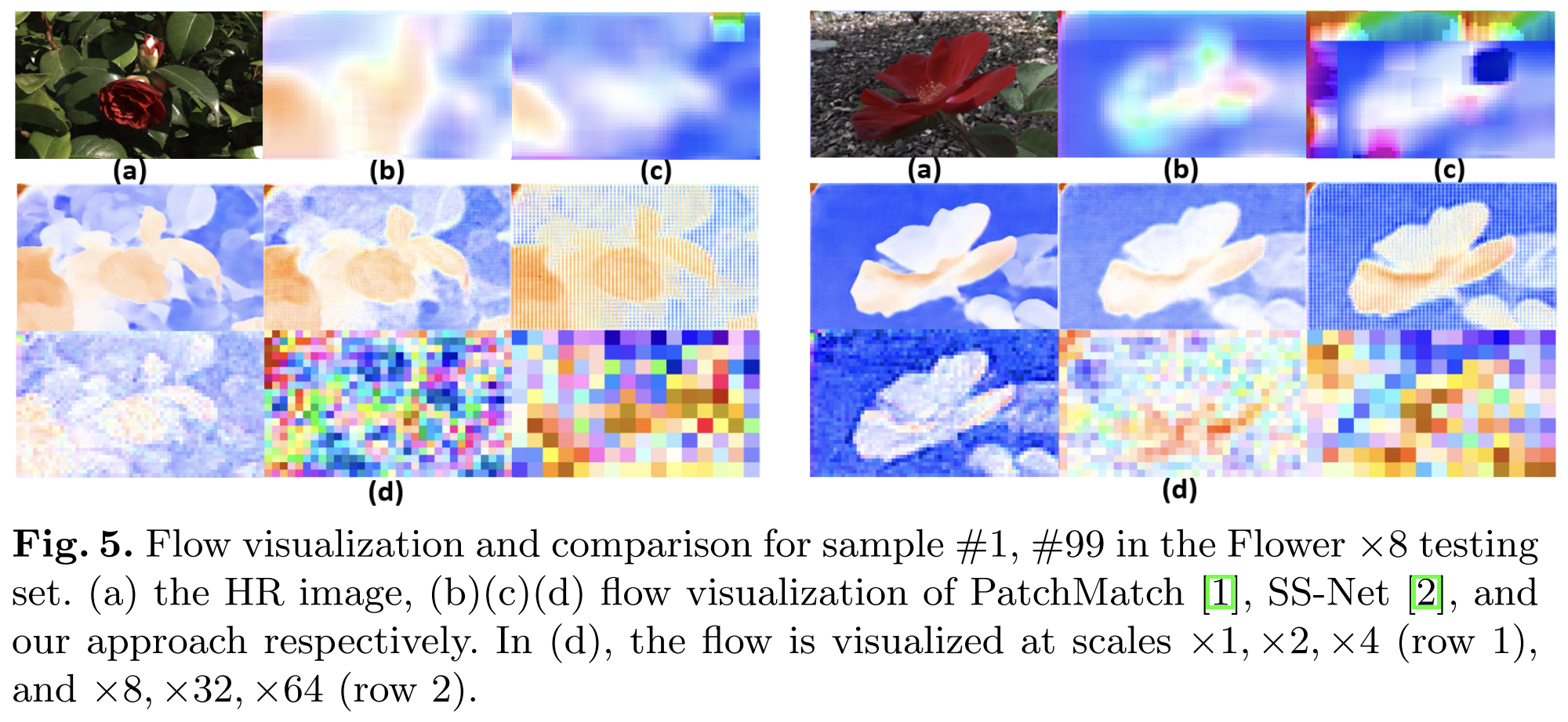
- Flows at scale 0–3 were coherent (good).
- Flows at scale 4–5 were too noisy — because those very small maps (like 32×32) lost too much information.
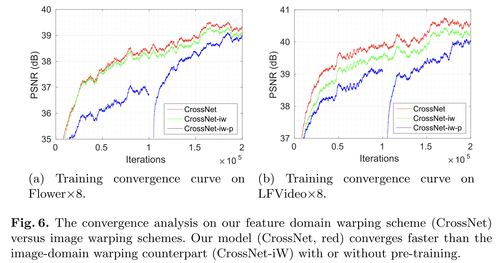
Training setup:
- Train both CrossNet and CrossNet-iw with the same procedure:
- Pre-train on LFVideo dataset
- Fine-tune on Flower dataset
- 200 K iterations total
- Additionally, CrossNet-iw pretraining:
- Pre-train only the flow estimator WS-SRNet using an image warping task for 100 K iterations.
- Train the whole network jointly for another 100 K iterations.
FlowNetS+ adds extra upsampling layers
- In the original FlowNetS:
- The final flow map is smaller than the input (maybe ¼ or ½ resolution).
- This is fine for rough alignment but loses small motion details.
- In FlowNetS+:
- They add extra upsampling layers so the final flow map is finer (closer to full size).
- That’s why it aligns better — it can describe tiny pixel movements more accurately.
Downsampling = make smaller. Upsampling = make bigger.