Abstract
The game of Go:
The most challenging of classic games for AI, because:
- Enormous search space
- The difficulty of evaluating board positions and moves
| Concept | Meaning | Example in Go | AI Solution |
|---|---|---|---|
| Enormous search space | Too many possible moves and future paths → impossible to explore all | At every turn, Go has ~250 legal moves; across 150 moves → (250^{150}) possibilities | Policy network narrows down the choices (reduces breadth of search) |
| Hard-to-evaluate positions | Even if you know the board, it’s hard to know who’s winning | Humans can’t easily assign a numeric score to a mid-game position | Value network predicts win probability (reduces depth of search) |
AlphaGo
Integrating deep neural networks with Monte Carlo Tree Search (MCTS).
The main innovations include:
- Two Neural Networks:
- Policy Network: Selects promising moves → the probability of each move.
- Value Network: Evaluates board positions → the likelihood of winning.
- Training Pipeline:
- Supervised Learning (SL) from expert human games to imitate professional play.
- Reinforcement Learning (RL) through self-play, improving beyond human strategies.
- Integration with MCTS:
- Combines the predictive power of neural networks with efficient search.
- Reduces:
- breadth (number of moves to consider)
- depth (number of steps to simulate) of search.
Results:
- Without search, AlphaGo already played at the level of strong Go programs.
- With the neural-network-guided MCTS, AlphaGo achieved a 99.8% win rate against other programs.
- It became the first program ever to defeat a human professional Go player (Fan Hui, European champion) by 5–0.
Introduction
- Optimal value function $v^*(s)$
- For any game state $s$, there exists a theoretical function that tells who will win if both players play perfectly.
- Computing this function exactly means searching through all possible sequences of moves.
- Search space explosion
- Total possibilities ≈ $b^d$, where
- $b$: number of legal moves (breadth),
- $d$: game length (depth).
- For Go: ( $b$ ≈ 250, $d$ ≈ 150) → bigggg number → impossible to compute exhaustively.
- Total possibilities ≈ $b^d$, where
- Reducing the search space — two key principles:
- (1) Reduce depth using an approximate value function $v(s)$:
- Stop (truncate) deep search early.
- Use an approximate evaluator to predict how good a position is instead of exploring all future moves.
- This worked in chess, checkers, and Othello, but was believed to be impossible (“intractable”) for Go because Go’s positions are much more complex.
- (2) Reduce breadth using a policy $p(a|s)$:
- Instead of exploring all moves, only sample the most likely or promising ones.
- This narrows down which actions/moves to consider, saving enormous computation.
- Example: Monte Carlo rollouts:
- Simulate random games (using the policy) to estimate how good a position is.
- Maximum depth without branching at all, by sampling long sequences of actions for both players from a policy $p$.
- This method led to strong results in simpler games (backgammon, Scrabble), and weak amateur level in Go before AlphaGo.
- (1) Reduce depth using an approximate value function $v(s)$:
Monte Carlo Rollout
Monte Carlo rollout estimates how good a position is by:
- Starting from a given board position (s).
- Playing many simulated games to the end (using policy-guided moves → reduce breadth).
- Recording each game’s result (+1 for win, −1 for loss).
- Averaging all outcomes to estimate the win probability for that position.
$$ v(s) \approx \text{average(win/loss results from rollouts)} $$
Goal:
Approximate the value function $v(s)$, the expected chance of winning from position $s$.
It’s simple but inefficient — great for small games, too slow and noisy for Go.
Monte Carlo tree search
- MCTS uses Monte Carlo rollouts to estimate the value of each state.
- As more simulations are done, the search tree grows and values become more accurate.
- It can theoretically reach optimal play,
- but earlier Go programs used shallow trees and simple, hand-crafted policies or linear value functions (not deep learning).
- These older methods were limited because Go’s search space was too large.
Training pipeline of AlphaGo
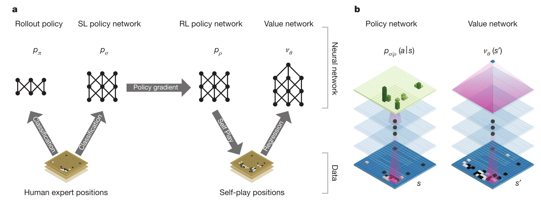
- Supervised Learning (SL) Policy Network $p_\sigma$:
- trained from human expert games.
- Fast Policy Network $p_\pi$:
- used to quickly generate moves during rollouts.
- Reinforcement Learning (RL) Policy Network $p_\rho$:
- improves the SL policy through self-play, optimizing for winning instead of just imitating humans.
- Value Network $v_\theta$:
- predicts the winner from any board position based on self-play outcomes.
- Final AlphaGo system = combines policy + value networks inside MCTS for strong decision-making.
Supervised learning of policy networks
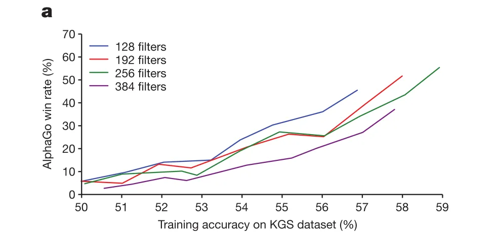
Panel(a): Better policy-network accuracy in predicting expert moves → stronger actual gameplay performance.
This proves that imitation learning (supervised policy $p_σ$) already provides meaningful playing ability before any reinforcement learning or MCTS.
Fast Rollout Policy networks
- A simpler and faster version of the policy network used during rollouts in MCTS.
- Uses a linear softmax model on small board-pattern features (not deep CNN).
- Much lower accuracy (24.2 %)
- but extremely fast
- takes only 2 µs per move (vs. 3 ms for the full SL policy).
- Trained with the same supervised learning principle on human moves.
Reinforcement learning of policy networks
- Structure of the policy network = SL policy network
- initial weights ρ = σ
| Step | What happens | What’s learned |
|---|---|---|
| Initialize | Copy weights from SL policy (ρ = σ) | Start with human-like play |
| Self-play | Pick current p and an older version p | Generate thousands of full games (self-play) |
| Reward | +1 for win, −1 for loss | Label each move sequence, and collect experience (state, action, final reward) |
| Update | Update weights ρ by SGD | Policy network |
| Repeat | Thousands of games | Stronger, self-improving policy |
Reinforcement learning of value networks
| Step | What happens | What’s learned |
|---|---|---|
| Initialize | Start from the trained RL policy network; use it to generate self-play games | Provides realistic, high-level gameplay data |
| Self-play | RL policy network plays millions of games against itself | Produce diverse board positions and their final outcomes (+1 win / −1 loss) |
| Sampling | Randomly select one position per game to form 30 M independent (state, outcome) pairs | Avoids correlation between similar positions |
| Labeling | Each position (s) labeled with the final game result (z) | Links every board state to its real win/loss outcome |
| Training | Train the value network (v_θ(s)) by minimizing MSE | Learns to predict winning probability directly from a position |
| Evaluation | Compare against Monte Carlo rollouts (pπ, pρ) | Matches rollout accuracy with 15 000× less computation |
| Result | MSE ≈ 0.23 (train/test), strong generalization | Reliable position evaluation for use in MCTS |
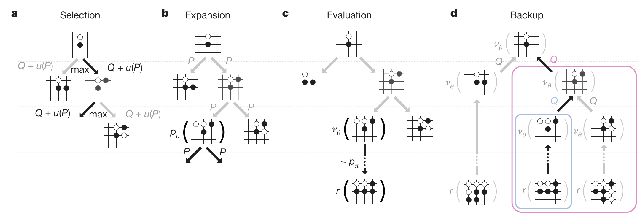
Searching with policy and value networks (MCTS)
| Panel | Step | What happens | Which network helps |
|---|---|---|---|
| a | Selection | Traverse the tree from root to a leaf by selecting the move with the highest combined score Q + u(P). | Uses Q-values (average win) and policy priors P (from policy network). |
| b | Expansion | When reaching a leaf (a position never explored before), expand it: generate its possible moves and initialize their prior probabilities using the policy network | RL policy network |
| c | Evaluation | Evaluate this new position in two ways: ① Value network (v_θ(s)): predicts win probability instantly. ② Rollout with fast policy p_π: quickly play random moves to the end, get final result (r). | Value net + Fast policy |
| d | Backup | Send the evaluation result (average of (v_θ(s)) and (r)) back up the tree — update each parent node’s Q-value (mean of all results from that branch). | None directly (update step) |
The core idea
Each possible move/edge (s, a) in the MCTS tree stores 3 key values:
| Symbol | Meaning | Source |
|---|---|---|
| P(s,a) | Prior probability — how promising this move looks before searching | From the policy network |
| N(s,a) | How many times this move has been tried | From search statistics |
| Q(s,a) | Average win rate from playing move a at state s | From past simulations |
Step 1: Selection — choose which move to explore next
At each step of a simulation, AlphaGo selects the move $a_t$ that maximizes:
$$ a_t = \arg\max_a [Q(s_t, a) + u(s_t, a)] $$
where the bonus term $u(s,a)$ encourages exploration:
$$ u(s,a) \propto \frac{P(s,a)}{1 + N(s,a)} $$
Step 2: Expansion
When the search reaches a leaf (a position not yet in the tree):
- The policy network $p_\sigma(a|s)$ outputs a probability for each legal move.
- Those values are stored as new P(s,a) priors for the new node.
- Initially
- $N(s,a) = 0$
- $Q(s,a) = 0$
Now the tree has grown — this new node represents a new possible future board.
Step 3: Evaluation — estimate how good the leaf is
Each leaf position $s_L$ is evaluated in two ways:
- Value network $v_θ(s_L)$: directly predicts win probability.
- Rollout result $z_L$: fast simulation (using the fast rollout policy $p_π$) until the game ends
- +1 if win
- −1 if loss.
Then AlphaGo combines the two results:
$$ V(s_L) = (1 - λ)v_θ(s_L) + λz_L $$
- $λ$ = mixing parameter (balances between value net and rollout).
- If $λ$ = 0.5, both count equally.
Step 4: Backup — update the tree statistics
The leaf’s evaluation $V(s_L)$ is propagated back up the tree:
Every move (edge) $(s, a)$ that was used to reach that leaf gets updated:
$$ N(s,a) = \sum_{i=1}^{n} 1(s,a,i) $$
$$ Q(s,a) = \frac{1}{N(s,a)} \sum_{i=1}^{n} 1(s,a,i) V(s_L^i) $$
So, Q(s,a) becomes the average value of all evaluations ( $r$ and $vθ$) in its subtree.
Step 5: Final move decision
After thousands of simulations, the root node has a set of moves with:
- $P(s_0, a)$: from policy network,
- $Q(s_0, a)$: average win rate,
- $N(s_0, a)$: visit counts.
AlphaGo chooses the move with the highest visit count (N) — the most explored and trusted move.
Implementation detail
- Evaluating policy & value networks takes much more compute than classical search.
- AlphaGo used:
- 40 search threads,
- 48 CPUs,
- 8 GPUs for parallel evaluation.
- The final system ran asynchronous multi-threaded search:
- CPUs handle the tree search logic,
- GPUs compute policy and value network evaluations in parallel.
This allowed AlphaGo to efficiently combine deep learning with massive search.
Discussion
- In this work we have developed a Go program, based on a combination of deep neural networks and tree search.
- We have developed, for the first time, effective move selection and position evaluation functions for Go,
- based on deep neural networks that are trained by a novel combination of supervised and reinforcement learning.
- We have introduced a new search algorithm that successfully combines neural network evaluations with Monte Carlo rollouts.
- Select those positions more intelligently, using the policy network, and evaluating them more precisely, using the value network.