Abstraction
CrossNet++ focuses on reference-based super-resolution (RefSR), improving a low-resolution image using a high-resolution reference from another camera. This task is hard because of large scale differences (8×) and big parallax (~10%) between the two views.
To solve this, CrossNet++ introduces an end-to-end two-stage network with:
- Cross-scale warping modules, align images at multiple zoom levels to narrow down parallax, handle scale and parallax differences.
- Image encoder and fusion decoder, extract multi-scale features and combine them to reconstruct a high-quality super-resolved image.
It uses new hybrid loss functions comprising warping loss, landmark loss and super-resolution loss to improve accuracy and stability by stabilizing the training of alignment module and helps to improve super-resolution performance.
1 Introduction
The development of method:
- patch-matching + patch-synthesis + iteratively applying non-uniform warping
Causes grid artifacts, incapable of handling the non-rigid image deformation- Directly warping between the low and high-resolution images is inaccurate.
- Such iterative combination of patch matching and warping introduces heavy computational burden.
- warping + synthesis
- It cannot effectively handle large-parallax cases that widely existed in real-world data.
- pre-warping + re-warping + synthesis
- CrossNet++ is a unified framework enabling fully end-to-end training which does not require pretraining the flow estimator.
- Two-stage pipeline: Two-stage cross-scale warping module.
- stage 1: Uses FlowNet to estimate motion (optical flow) between the low-resolution (LR) and reference (Ref) images without needing ground-truth flow (self-supervised). This produces a roughly aligned “warped-Ref” image.
- stage 2: Further refines alignment between the warped-Ref and LR image for more accurate warping.
- Hybrid loss: warping loss, landmark loss and super-resolution loss.
- warping loss: supervise the flow estimation implicitly.
- landmark loss: supervise the flow estimation explicitly.
2 Related Work
3 Preliminary of CrossNet
3.3 Network Structure
3.3.1 Alignment Module
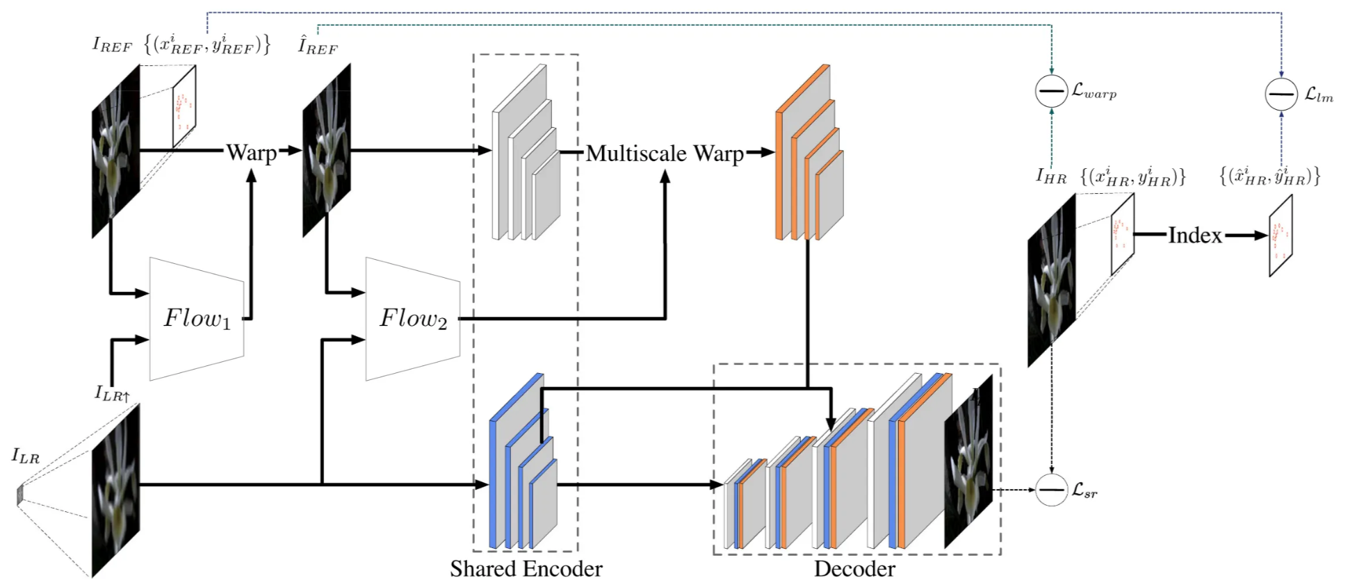
The alignment module aims to align the reference image $I_{REF}$ with the low-resolution image $I_{LR}$. CrossNet++ adopts a warping-based alignment using two-stage optical flow estimation.
In the first stage, a modified FlowNet (denoted as $Flow_1$) predicts the flow field between an upsampled LR image $I_{LR↑}$ and the reference image $I_{REF}$:
where $V_1^0$ represents the flow at scale 0 (the original image scale). The upsampled LR image $I_{LR↑}$ is obtained via a single-image SR method:
Then, the reference image is spatially warped using this flow to produce the pre-aligned reference:
In the second stage, the pre-aligned reference \( \hat{I}_{\mathrm{REF}} \) and the upsampled LR image \( I_{LR}\uparrow \) are again input to another flow estimator \( Flow_2 \) to compute multi-scale flow fields:
These multi-scale flows are used later in the synthesis network to refine alignment and reconstruct the final super-resolved image.
this two-stage alignment, coarse warping followed by multi-scale refinement—allows CrossNet++ to handle large parallax and depth variations, achieving more accurate correspondence and better alignment quality than the original CrossNet.
3.3.2 Encoder
Through the alignment module, we obtain four flow fields at different scales. The encoder receives the pre-aligned reference image $\hat I_{REF}$ and the upsampled LR image $I_{LR↑}$, then extracts their feature maps at four different scales.
The encoder has five convolutional layers with 64 filters of size ( 5 $\times$ 5 ).
- The first two layers (stride = 1) extract the feature map at scale 0.
- The next three layers (stride = 2) produce lower-resolution feature maps for scales 1 to 3.
These operations are defined as: where $\sigma$ is the ReLU activation, $*_1$ and $*_2$ denote convolutions with strides 1 and 2 respectively, and $F^i$ is the feature map at scale $i$.
Unlike the original CrossNet, CrossNet++ uses a shared encoder for both $\hat I_{REF}$ and $I_{LR↑}$ instead of two separate encoders, which reduces about 0.41 M parameters while maintaining accuracy.
The resulting feature sets are:
Finally, each reference feature map $F^i_{REF}$ is warped using the multi-scale flow fields $V^i_2$ from to produce the aligned feature maps:
In short, the encoder extracts multi-scale feature maps for both LR and reference images using shared convolutional layers, then aligns the reference features to the LR features through warping with multi-scale flow fields, which provides precise, scale-consistent alignment for the next fusion step.
3.3.3 Decoder
After feature extraction and alignment, the decoder fuses the LR and reference feature maps and generates the final super-resolved image.
It follows a U-Net-like structure, which progressively upsamples the feature maps from coarse to fine scales.
To create the decoder features at scale $i$, the model concatenates:
- the warped reference features $\hat{F}^i_{REF}$,
- the LR image features $F^i_{LR}$ ,
- and the decoder feature from the next coarser scale $F^{i+1}_{D}$ (if available).
Then a deconvolution layer (stride 2, filter size 4 $\times$ 4) is applied:
where $*_2$ is deconvolution with stride 2 and $\sigma$ is the activation (ReLU).
After that, three more convolutional layers (filter sizes (5 $\times$ 5), channels {64, 64, 3}) perform post-fusion to synthesize the final image $I_p$:
where $*_{1}$ means convolution with stride 1.
The decoder takes aligned multi-scale features from LR and reference images, fuses them step by step through deconvolutions and convolutions, and finally reconstructs the high-resolution output image $I_p$, the sharp, super-resolved result.
3.4 Loss Function
warping loss, landmark loss → encourage flow estimator to generate precise flow.
super-resolution loss → is responsible for the final synthesized image.
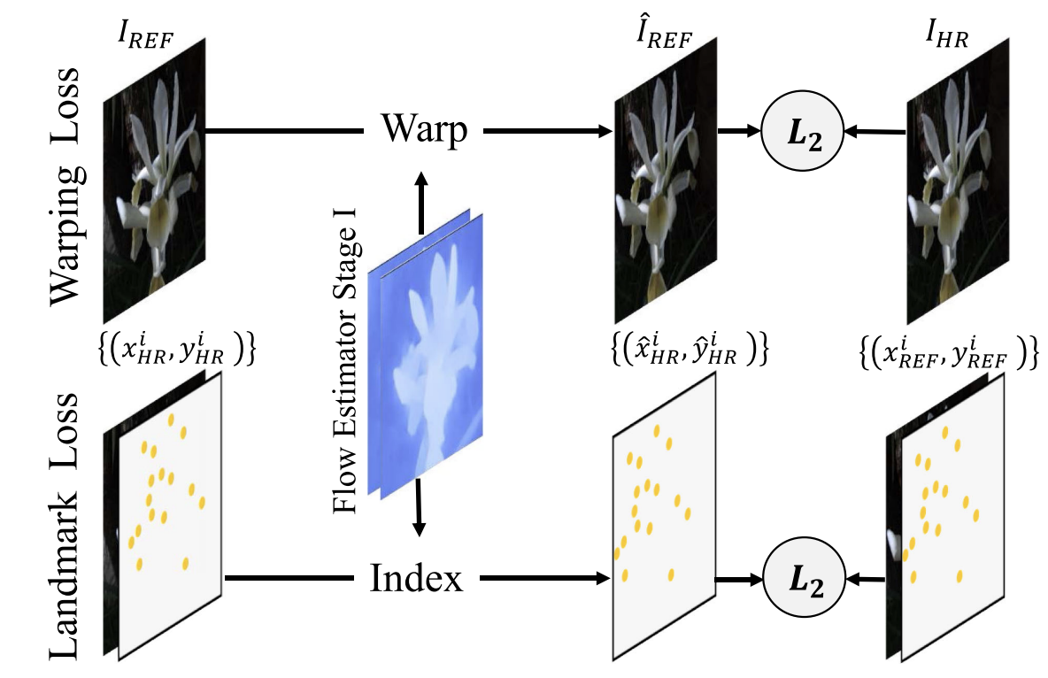
3.4.1 Warping Loss
Used in the first-stage Flow Estimator to regularize the generated optical flow.
It ensures that the warped reference image $\hat I_{REF}$ is close to the ground-truth HR image $I_{HR}$, assuming both share a similar viewpoint.
The loss minimizes pixel-wise intensity differences:
where $N$ is the total number of samples, $i$, $s$, and $c$ iterate over training samples, spatial locations and color channels respectively.
3.4.2 Landmark Loss
This loss provides directional geometric guidance for large-parallax cases.
It uses SIFT feature matching to find corresponding landmark pairs $(p, q)$ between the HR and reference images, and applies the flow field $V^0_1$ to warp these landmarks.
The warped landmark $\hat{p}^j$ is computed as:
and the landmark loss penalizes the distance between warped and target landmarks:
where $m_i$ is the number of landmark pairs in image $i$.
This term helps the flow estimator predict more accurate motion fields, especially when viewpoints differ greatly.
3.4.3 Super-Resolution Loss
This loss directly trains the model to synthesize the final super-resolved image $I_p$, comparing it with the ground-truth high-resolution image $I_{HR}$ using the Charbonnier penalty (a smooth $L_1$ loss):
4 Experiment
Flower dataset and LFVideo dataset
- 14 $\times$ 14 angular samples of size 376 $\times$ 541.
- training and testing:
- central 8 $\times$ 8 grid of angular samples
- top-left 320 $\times$ 512 for training and testing
- training: 3243 images from Flower and 1080 images from LFVideo
- testing: 100 images from Flower and 270 images from LFVideo