Abstraction
Bayesian Optimization is a method for finding the best solution when evaluating the objective function is slow or expensive (taking minutes or hours).
It is mainly used for problems with fewer than 20 variables and where evaluations may contain noise.
The method works by:
- Building a surrogate model of the unknown function using a Bayesian machine learning method called Gaussian Process regression, which predicts both the function value and its uncertainty.
- Using an acquisition function (expected improvement, knowledge gradient or entropy search) to decide where to sample next — balancing exploration and exploitation.
The tutorial also extends expected improvement to handle noisy evaluations, supported by a formal decision-theoretic argument, rather than ad hoc fixes.
1 Introduction
Bayesian Optimization (BayesOpt) is a machine learning–based method for optimizing expensive, black-box functions, it’s designed for black-box derivative-free global optimization. It aims to solve
$$ \max_{x \in A} f(x) $$
where $f(x)$ is expensive to evaluate, derivative-free, and continuous.
| Concept | Meaning | Intuition |
|---|---|---|
| Search space | The entire region of possible inputs x, its dimensionality tells us how complex the problem is. | it’s the multi-dimensional space that defines where you can look. |
| Feasible set / search area | The subset of that space that you actually allow x to take, i.e., with all constraints applied. | this is the region inside the search space that satisfies all limits (bounds, rules). |
BayesOpt is for global optimization of black-box functions. It builds a surrogate model of f(x) using a Bayesian machine learning technique, typically Gaussian Process (GP) regression. It then chooses where to sample next using an acquisition function (e.g., Expected Improvement, Knowledge Gradient, or Entropy Search). This balances exploration (trying uncertain areas) and exploitation (sampling promising areas).
The ability to optimize expensive black-box derivative-free functions makes BayesOpt extremely versatile. Recently it has become extremely popular for tuning hyperparameters in machine learning algorithms. And it’s also suitable for engineering design, scientific experiments and reinforcement Learning.
What makes Bayesian Optimization unique compared to general surrogate-based optimization approaches are using surrogates developed using bayesian statistics and choosing new points using a probabilistic acquisition rule instead of heuristics. (reasoning probabilistically about what it already knows and what it’s uncertain about)
2 Overview of BayesOpt
BayesOpt consists of two main components: a Bayesian statistical model for modeling the objective function, and an acquisition function for deciding where to sample next.
- Bayesian Statistical Model
Models the unknown objective function $f(x)$.
Typically a Gaussian Process (GP).
Produces a posterior distribution:
$$ f(x) \sim \mathcal{N}(\mu_n(x), \sigma_n^2(x)) $$
where:
- $\mu_n(x)$: predicted mean (best guess)
- $\sigma_n(x)$: predicted uncertainty
Updated each time new data (evaluations of f) are observed.
- Acquisition Function
- Decides where to sample next based on the GP’s posterior.
- Measures the “value” of sampling a new point x:
- High $\mu_n(x)$: promising area.
- High $\sigma_n(x)$: uncertain area.
- Common types: Expected Improvement (EI), Knowledge Gradient (KG), Entropy Search (ES), and Predictive Entropy Search (PES).
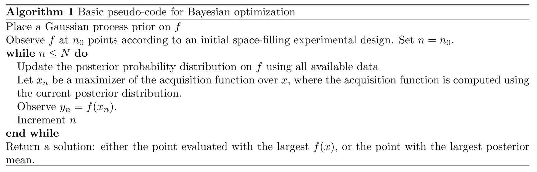
After evaluating the objective according to an initial space-filling experimental design, often consisting of points chosen uniformly at random, they are used iteratively to allocate the remainder of a budget of N function evaluations.
3 Gaussian Process (GP) Regression
Gaussian Process (GP) Regression is a Bayesian way to model an unknown function $f(x)$.
It assumes that any collection of function values $[f(x_1), f(x_2), …, f(x_k)]$ follows a multivariate normal distribution with a specific mean vector and covariance matrix.
So instead of guessing one possible curve for $f(x)$, we assume a probability distribution over all possible smooth curves.
3.1 Initialization Steps
Step 1: Define the Prior
Before we see any data, we describe our belief about $f(x)$ using:
- A mean function $\mu_0(x)$ → gives the average expected value, often set to 0 (no bias).
- A covariance (kernel) function $\Sigma_0(x_i, x_j)$ → shows how similar two points are.
- Close points = high correlation (similar f values)
- Far points = low correlation (independent values)
Together, they form the prior:
$$ f(x_{1:k}) \sim \text{Normal}(\mu_0(x_{1:k}), \Sigma_0(x_{1:k}, x_{1:k})) $$
Step 2: Update with Observed Data (Bayes’ Rule)
Once we have some known data $(x_1, f(x_1)), …, (x_n, f(x_n))$, we update our belief to get the posterior distribution, what we now believe about the function after seeing real values.
For a new point x:
$$ f(x)|f(x_{1:n}) \sim \text{Normal}(\mu_n(x), \sigma_n^2(x)) $$
where:
- $\mu_n(x)$: the posterior mean — our best prediction at $x$
- $\sigma_n^2(x)$: the posterior variance — how uncertain we are at $x$
The GP uses the kernel to decide how much nearby points influence the prediction:
- If $x$ is near known points → high confidence, low uncertainty.
- If $x$ is far from all known points → low confidence, high uncertainty.
Step 3: Posterior Formula
$$ \mu_n(x) = \Sigma_0(x, x_{1:n})\Sigma_0(x_{1:n}, x_{1:n})^{-1}(f(x_{1:n}) - \mu_0(x_{1:n})) + \mu_0(x) $$
$$ \sigma_n^2(x) = \Sigma_0(x, x) - \Sigma_0(x, x_{1:n})\Sigma_0(x_{1:n}, x_{1:n})^{-1}\Sigma_0(x_{1:n}, x) $$
Meaning:
- The new prediction $\mu_n(x)$ = weighted average of nearby known values (old belief + weighted correction from known data)
- The uncertainty $\sigma_n^2(x)$ = initial uncertainty minus what we’ve learned (reduce uncertainty)
Step 4: Practical Notes
- Instead of directly inverting large matrices, use Cholesky decomposition for stability and speed.
- Add a tiny number (e.g., $10^{-6}$) to the diagonal of the covariance matrix to prevent numerical errors.
- The same formulas work for:
- Many new points at once (matrices)
- Continuous domains (theoretically infinite points)
3.2 Choosing a Mean Function and Kernel
Kernel choice
The kernel (covariance function) defines how much two inputs (x) and (x’) are correlated. Points that are close in the input space are more strongly correlated, the kernel must be positive semi-definite (it cannot give negative variances):
$$ if (||x - x’|| < ||x - x’’||), then (Σ_0(x, x’) > Σ_0(x, x’’)). $$
Power Exponential (Gaussian) Kernel
$$ Σ_0(x, x’) = α_0 \exp(-||x - x’||^2) $$
The is the most common kernel and produces very smooth functions.
- $α_0$ controls overall variance (how much $f(x)$ can vary).
- $α_i$ inside $||x - x’||^2 = \sum_i α_i (x_i - x’_i)^2$ control how quickly correlation decreases as inputs differ.
Matérn Kernel
$$ Σ_0(x, x’) = α_0 \frac{2^{1-ν}}{Γ(ν)} (\sqrt{2ν}||x - x’||)^{ν} K_ν(\sqrt{2ν}||x - x’||) $$
- Adds a parameter $ν$ that controls smoothness.
- Smaller $ν$ produces rougher functions, larger $ν$ gives smoother ones.
- $K_ν$ is the modified Bessel function.
Mean function
The mean function expresses the expected trend of $f(x)$ before seeing data. The most common choice is a constant mean: $μ_0(x) = μ$. And If $f(x)$ is believed to have a trend, a parametric mean can be used:
$$ μ_0(x) = μ + \sum_{i=1}^{P} β_i Ψ_i(x) $$
where $Ψ_i(x)$ are basis functions, often low-order polynomials.
For example, $Ψ(x) = x$ gives a linear trend, $Ψ(x) = [1, x, x^2]$ gives a quadratic trend.
3.3 Choosing Hyperparameters
The mean and kernel functions contain parameters (like $\alpha_0, \nu, \mu$) called hyperparameters, grouped in a vector $\eta$. These control how the Gaussian Process behaves (for example, how smooth it is or what its average level is).
Maximum Likelihood Estimation (MLE)
$$ \hat{\eta} = \arg\max_{\eta} P(f(x_{1:n}) | \eta) $$
Choose hyperparameters that make the observed data most likely under the GP model. It’s simple and widely used. But it can give unreasonable results if the model overfits (e.g., too smooth or too wiggly).
Maximum a Posteriori (MAP)
$$ \hat{\eta} = \arg\max_{\eta} P(\eta | f(x_{1:n})) = \arg\max_{\eta} P(f(x_{1:n}) | \eta) P(\eta) $$
Similar to MLE, but adds a prior $P(\eta)$ on the hyperparameters. This prior prevents extreme or unrealistic parameter values. The MLE is a special case of MAP when $P(\eta)$ is constant (flat). Common priors include uniform, normal, or log-normal distributions.
Fully Bayesian Approach
$$ P(f(x) = y| f(x_{1:n})) = \int P(f(x) = y| f(x_{1:n}), \eta) P(\eta | f(x_{1:n})) d\eta $$
Instead of choosing a single best $\eta$, it integrates over all possible values of the hyperparameters. It produces more robust uncertainty estimates but is computationally expensive. In practice, it’s approximated using sampling methods (e.g., MCMC). MAP can be viewed as an approximation to this full Bayesian inference.
Don’t fix η; instead, consider all possible η, weighted by how likely each one is.
But this high-dimensional and usually cannot be computed exactly, so in practice, we approximate it by sampling:
$$ P(f(x) = y |f(x_{1:n})) \approx \frac{1}{J} \sum_{j=1}^{J} P(f(x) = y |f(x_{1:n}), \eta = \eta_{j}) $$
where the samples $\eta_j$ are drawn from $P(\eta | f(x_{1:n}))$. This is typically done using MCMC (Markov Chain Monte Carlo).
3. Summary table
| Method | In short | Pros | Cons |
|---|---|---|---|
| MLE | Fit the data best | Finds hyperparams that best fit data | Simple |
| MAP | Fit the data but stay reasonable | Adds prior to control extremes | More stable |
| Fully Bayesian | Consider all possible fits, weighted by probability | computationally expensive | Integrates over all possible scenarios |
4 Acquisition Functions
Expected Imrpvement(EI), Knowledge Gradient(KG), Entropy Search(ES)
4.1 Expeced Improvement
Goal: Decide where to sample next so that we are likely to improve our current best result.
Suppose we have already tested n points. The best value so far is
$$ f_n^* = \max_{m \le n} f(x_m) $$
If we evaluate a new point x, its value f(x) is uncertain. The improvement is how much better it is than the current best:
$$ I(x) = [f(x) - f_n^*]^+ = \max(f(x) - f_n^*, 0) $$
Since f(x) is a random variable under the Gaussian Process model, we take the expected value of this improvement:
$$ EI_n(x) = E_n[[f(x) - f_n^*]^+] $$
Because $f(x) \sim \mathcal{N}(\mu_n(x), \sigma_n^2(x))$, EI can be computed in closed form:
$$ EI_n(x) = (\mu_n(x) - f_n^*)\Phi(z) + \sigma_n(x)\phi(z), \quad z = \frac{\mu_n(x) - f_n^*}{\sigma_n(x)} $$
where $\Phi$ is the normal CDF and $\phi$ is the normal PDF.
$Φ(z)$ = the cumulative distribution function (CDF) of the standard normal.
→ It gives the probability that a standard normal variable is ≤ z.
$ϕ(z)$ = the probability density function (PDF) of the standard normal.
→ It gives the height of the bell curve at z.
The next sampling point is chosen by maximizing EI:
$$ x_{n+1} = \arg\max_x EI_n(x) $$
Interpretation:
EI balances two goals:
- Exploitation: sampling where the predicted mean $\mu_n(x)$ is high.
- Exploration: sampling where uncertainty $\sigma_n(x)$ is high.
This trade-off helps the algorithm explore new areas and improve known good ones efficiently.
4.2 Knowledge Gradient
The Knowledge Gradient (KG) acquisition function measures the expected value of information gained from sampling a new point.
Unlike Expected Improvement (EI), which focuses on immediate improvement at the sampled point, KG evaluates how much better our overall knowledge about the objective becomes after sampling.
- EI assumes the final solution must be one of the evaluated points.
- KG relaxes this: after we take one more sample, we can still choose any point (evaluated or not) as our final decision.
- Therefore, the value of sampling comes not just from finding a better local result, but from improving the entire model’s understanding of the objective surface.
Mathematical Form:
$$ KG_n(x) = E_n[\mu_{n+1}^* - \mu_n^*] $$
where
- $\mu_n^* = \max_{x’} \mu_n(x’)$: current predicted maximum,
- $\mu_{n+1}^* = \max_{x’} \mu_{n+1}(x’)$: predicted maximum after taking a new sample at (x),
- The expectation $\mathbb{E}_n[\cdot]$ averages over possible outcomes of the new observation.
Interpretation:
KG measures the expected increase in the best achievable posterior mean after taking one new sample.
Algorithm 2 Simulation-based computation
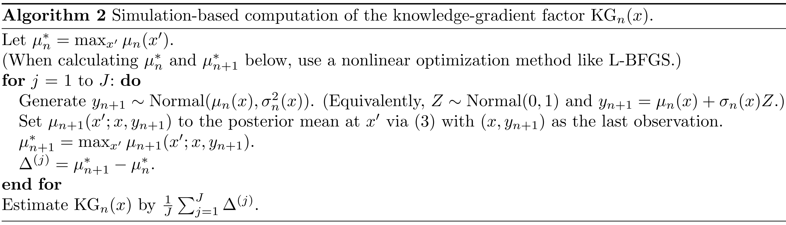
Purpost: estimate how much the best mean prediction might improve if we sample at x.
Steps:
Find the current best mean value
$$ \mu_n^* = \max_{x’} \mu_n(x’) $$
This is the best prediction under the current Gaussian Process (GP).
Simulate what could happen if we sample at x
Repeat J times (Monte Carlo simulation):
Draw a random possible observation
$$ y_{n+1} \sim \mathcal{N}(\mu_n(x), \sigma_n^2(x)) $$
(equivalently, $y_{n+1} = \mu_n(x) + \sigma_n(x)Z ; Z\sim\mathcal{N}(0,1)$).
Update the GP posterior using this “imagined” observation $(x, y_{n+1})$, obtaining a new mean function $\mu_{n+1}(\cdot)$.
Compute the new best mean value
$$ \mu_{n+1}^* = \max_{x’} \mu_{n+1}(x’) $$
Compute the gain for this scenario
$$ \Delta^{(j)} = \mu_{n+1}^* - \mu_n^* $$
Average over all J simulations
The Knowledge Gradient estimate is
$$ KG_n(x) = \frac{1}{J}\sum_{j=1}^J \Delta^{(j)} $$
Algorithm 3: Multi-start Stochastic Gradient Ascent
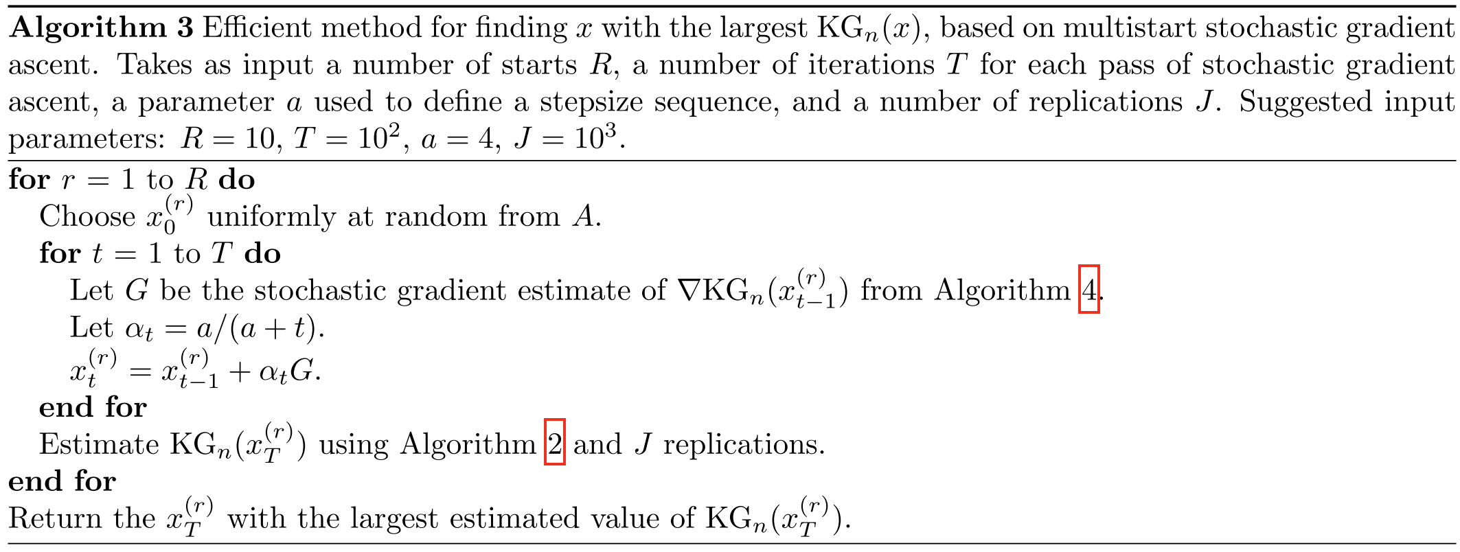
Goal: Find the best next sampling point $x$ that maximizes $KG_n(x)$.
Process:
Start from multiple random initial points $x_0^{(r)}$ (r = 1,…,R).
For each start, perform T stochastic gradient ascent steps:
Compute stochastic gradient $G$ (estimated using Algorithm 4).
Update $x_t^{(r)} = x_{t-1}^{(r)} + \alpha_t G$,
where $\alpha_t = a / (a + t)$ is a decreasing step size.
After T steps, estimate $KG_n(x_T^{(r)})$ using simulation (Algorithm 2).
Return the point with the largest estimated KG value.
Notes:
- Using multiple random starts helps avoid local optima.
- This method converges to a local maximum of the KG function.
Algorithm 4 — Simulation of Stochastic Gradients
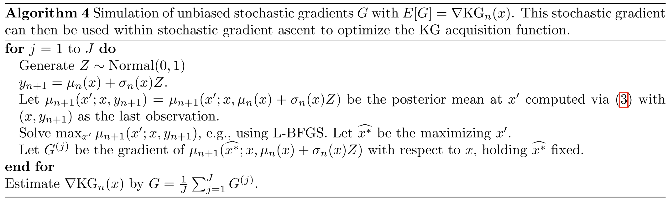
Purpose: Compute an unbiased estimate of the gradient $\nabla KG_n(x)$.
Steps:
- For each of J simulations:
- Sample a random variable $Z \sim \mathcal{N}(0,1)$.
- Generate a possible observation $y_{n+1} = \mu_n(x) + \sigma_n(x)Z$.
- Update the GP posterior using $(x, y_{n+1})$ to obtain new mean $\mu_{n+1}$.
- Compute the new best posterior mean value $\mu^*{n+1} = \max{x’} \mu{n+1}(x’)$.
- Evaluate its gradient w.r.t. the sampled point x.
- Average over all J samples to estimate $\nabla KG_n(x)$.
4.3 Entropy Search and Predictive Entropy Search
Entropy Search (ES) and Predictive Entropy Search (PES) are acquisition functions in Bayesian optimization that try to reduce uncertainty about the position of the global optimum $x^*$.
Instead of asking “which point will improve the function value most,” they ask “which point will tell me the most about where the best value is.”
Entropy Search (ES)
Purpose: Measures how much uncertainty (entropy) about the true optimum $x^*$ will go down if we sample at point x.
- $P_n(x^*)$: the current posterior belief over where the global optimum lies.
- $H(P_n(x^*))$: its entropy, representing uncertainty.
- After sampling at a candidate point x, the posterior changes to $P_n(x^*|f(x))$.
- The expected reduction in entropy is
$$ ES_n(x) = H(P_n(x^*)) - E_{f(x)}[H(P_n(x^*|f(x)))] $$
This means we prefer points x where observing $f(x)$ is expected to most reduce our uncertainty about $x^*$. Computing ES directly is difficult, because it requires calculating entropy over many possible function outcomes.
Predictive Entropy Search (PES)
Purpose: Measures how much uncertainty (entropy) about the true optimum $x^*$ will go down if we sample at point x.
PES reformulates the same idea in a simpler way. Instead of measuring the entropy of the optimum location directly, it measures the mutual information between $f(x)$ and $x^*$:
$$ PES_n(x) = H(P_n(f(x))) - \mathbb{E}_{x^*}[H(P_n(f(x)|x^*))] $$
This is mathematically equivalent to ES but easier to approximate in practice. PES estimates how much knowing the value of $f(x)$ would reduce uncertainty about where the optimum is.
Entropy Search and Predictive Entropy Search choose sampling points that give the most information about the global optimum.
They are more global and information-driven than EI or KG but are computationally more complex.
4.4 Multi-Step Optimal Acquisition Functions
Bayesian optimization can be viewed as a sequential decision process: each sample depends on past results. Standard methods like EI, KG, ES, and PES are one-step optimal, choosing the next point assuming only one evaluation remains.
A multi-step optimal strategy would plan several future evaluations ahead, maximizing total expected reward. However, computing it is extremely hard due to the dimensionality.
Recent studies have tried approximate multi-step methods using reinforcement learning and dynamic programming, but they are not yet practical. Experiments show that one-step methods already perform nearly as well, so they remain the preferred approach in practice.
5 Exotic Bayesian Optimization
Noisy Evaluations
Gaussian Process (GP) regression can handle noisy observations by adding noise variance to the covariance matrix. In practice, the noise variance is often unknown and treated as a hyperparameter. If noise varies across the domain, it can be modeled with another GP.
Acquisition functions like EI, KG, ES, and PES naturally extend to noisy settings, but EI becomes less straightforward since the “improvement” is not directly observable. The KG approach is more robust under noise.
Parallel Evaluations
Parallel Bayesian optimization allows evaluating several points simultaneously using multiple computing resources. Expected Improvement (EI) is extended to parallel EI, where several points $(x^{(1)}, \dots, x^{(q)})$ are selected jointly to maximize expected improvement.
Variants like multipoint EI and Constant Liar approximations simplify optimization. Similar extensions exist for KG, ES, and PES. Parallel versions are computationally harder but useful for speeding up optimization on modern systems.
Constraints
In real problems, sampling may be limited by constraints $g_i(x) \ge 0$ (g is the constraint). These constraints can be as expensive to evaluate as $f(x)$. EI can be extended to check improvement only among feasible points, i.e., points that satisfy all $g_i(x) \ge 0$.
Recent work also studied constrained Bayesian optimization under noisy or uncertain feasibility.
Multi-Fidelity and Multi-Information Source Evaluations
Sometimes there are multiple ways to estimate the objective, each with different accuracy and cost (called fidelities). For example, $f(x, s)$ may represent evaluating $x$ with fidelity level $s$:
- low fidelity is cheap but inaccurate
- high fidelity is expensive but precise
The goal is to allocate a limited total budget among fidelities to maximize information gain. Methods like KG, ES, and PES can handle this setting, but EI does not generalize well because evaluating $f(x, s)$ for $s ≠ 0$ never provides an improvement in the best objective function value seen.
Random Environmental Conditions and Multi-Task Bayesian Optimization
Here, the objective $f(x, w)$ depends on both design variables x and random environmental variables w (e.g., weather, test fold, etc.). The aim is to optimize either the expected value $\int f(x,w)p(w)dw$ or the sum over tasks $\sum f(x,w)p(w)$.
By observing performance under different w, we can infer information about nearby conditions, reducing the need for full evaluations. This setup is widely used in engineering, machine learning (cross-validation folds), and reinforcement learning. Modified EI, KG, and PES methods apply here.
Derivative Observations
Sometimes gradient (derivative) information is available along with function values. Gradients can be incorporated into GP models to improve predictions and optimization speed. While EI does not directly benefit from derivatives, KG can use them effectively.
Gradient-based updates improve convergence and numerical stability, especially in regions where function evaluations are expensive.
6 Software
7 Conclusion and Research Directions
7.1 Conclusion
The paper reviews Bayesian Optimization (BO) including Gaussian Process (GP) regression, and key acquisition functions such as expected improvement (EI), knowledge gradient (KG), entropy search (ES), and predictive entropy search (PES). And paper extends discussion to more complex cases (noise, constraints, multi-fidelity, multi-task, etc.).
7.2 Future Research Directions
- Theory and Convergence:
- There is a need for a deeper theoretical understanding of BO.
- Multi-step optimal algorithms are known to exist but are hard to compute.
- We lack finite-time performance guarantees and full understanding of convergence rates.
- Beyond Gaussian Processes:
- Most BO methods use GPs, but new statistical models may better capture some types of problems.
- Research should aim to develop alternative models suited for specific applications.
- High-Dimensional Optimization:
- Current BO struggles when the number of parameters is large.
- New methods should leverage structure in high-dimensional problems.
- Exotic Problem Structures:
- BO should handle more complex, real-world conditions (multi-fidelity data, environmental randomness, derivative information).
- Combining method development with practical applications can reveal new challenges and innovations.
- Real-World Impact:
- BO has strong potential in chemistry, materials science, and drug discovery, where experiments are expensive and slow.
- However, few researchers in these fields currently use BO — so expanding awareness and applications is important.