Introduction
Most models (RNNs, CNNs, Transformers) cannot handle very long sequences well. They either forget, see too little context, or are too slow. This makes long-range dependency tasks hard to solve.
State Space Models (SSMs) can solve this issue by remembering long information. But the old version (LSSL) used too much time and memory, so it was not practical.
New solution S4 fixes this by changing how the SSM is built. It splits the main matrix into simple parts and computes in a faster, more stable way. Now it runs much faster and uses much less memory.
Background: State Spaces
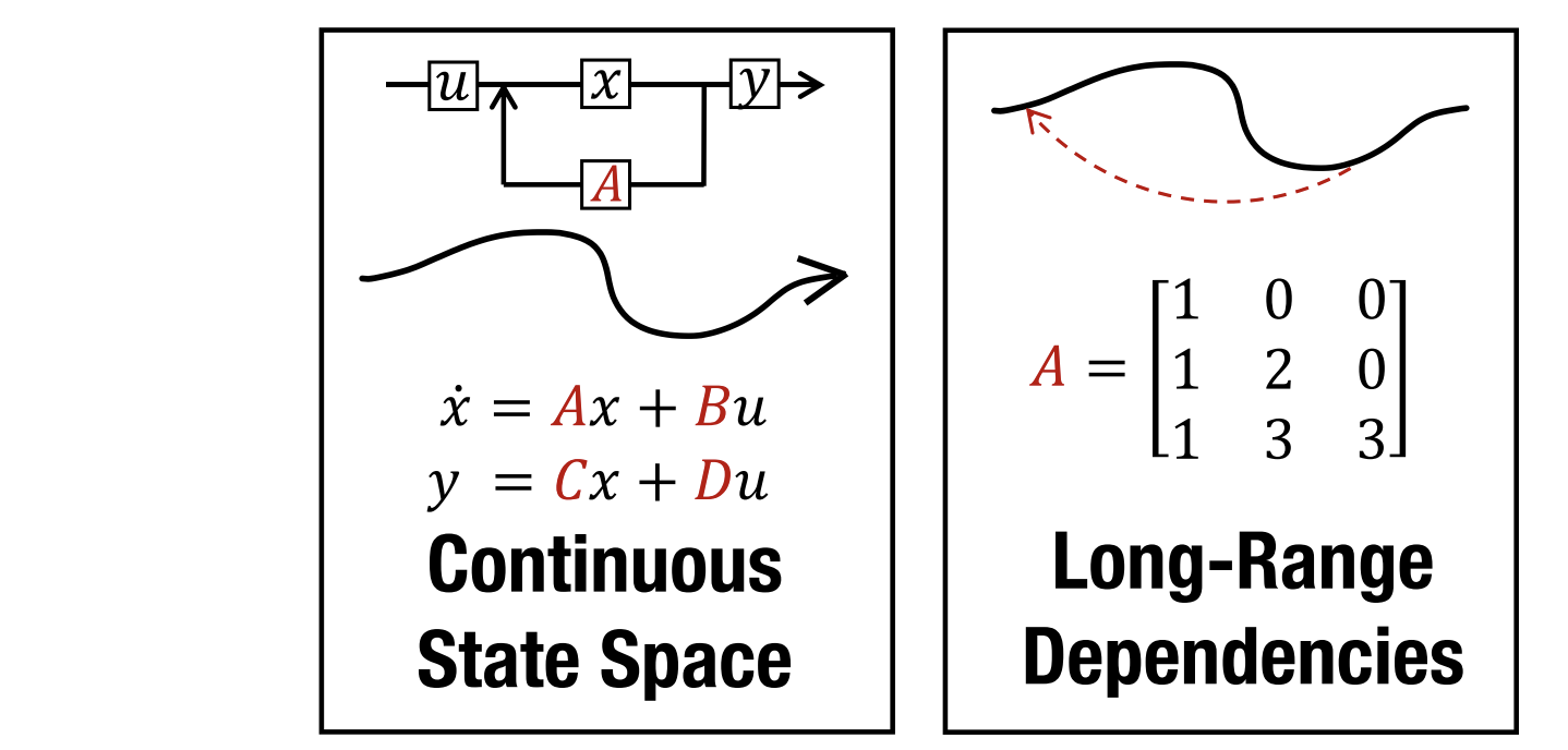
State Space Models (SSMs) describe how input changes hidden states and produces output. They learn parameters A, B, C, D automatically. Usually, D is ignored because it’s just a shortcut.
$$ x’(t) = A x(t) + B u(t) \\ y(t) = C x(t) + D u(t) $$
The basic SSM forgets or explodes on long sequences. HiPPO fixes this by giving a special matrix for A that helps the model remember long-term information.
$$ A_{nk} = \begin{cases} -(2n + 1)^{1/2}(2k + 1)^{1/2}, & \text{if } n > k \\ -(n + 1), & \text{if } n = k \\ 0, & \text{if } n < k \end{cases} $$
Real data comes in steps, so the SSM is turned into a discrete version that works like an RNN. To train faster, the model is rewritten as a convolution, which processes all inputs in parallel. The convolution weights are called the SSM kernel (K). (More details move to More Details)
Method: Structured State Spaces (S4)
S4 is a new way to make State Space Models (SSMs) fast and stable. The technical results focus on developing the S4 parameterization and showing how to efficiently compute all views of the SSM. It connects three forms of SSMs — continuous, recurrent, and convolutional — in one model.
The old method was slow because it multiplied a big matrix many times. S4 fixes this by rewriting the matrix as Normal + Low-Rank, which is easier to compute. This design makes S4 very efficient:
- Recurrent form: O(N) time per step
- Convolution form: O(N + L) total time
Each S4 layer has trainable parts (Λ, P, Q, B, C) and works like a CNN or Transformer layer. Stacking layers with activations makes it powerful for long-sequence data.
$$ A = V \Lambda V^{} - P Q^{\top} = V \left( \Lambda - (V^{}P)(V^{}Q)^{} \right) V^{*} $$
Conclusion
S4 is based on the State Space Model (SSM), which works like an RNN — it keeps a hidden state and updates it over time.
The problem with the old version is that the state update matrix A is hard to compute and unstable for long sequences. S4 solves this by rewriting A into a new, easier form:
$$ A = V \Lambda V^{*} - P Q^{\top} $$
This form (called Normal + Low-Rank) makes A stable, efficient, and fast to compute. As a result, S4 keeps the good memory ability of RNNs but runs much faster and handles much longer sequences.
More Details
Step 1: The original state space equations
Continuous-time form:
$$ x’(t) = A x(t) + B u(t) $$
$$ y(t) = C x(t) $$
Discrete-time version (after discretization):
$$ x_k = \bar{A} x_{k-1} + \bar{B} u_k $$
$$ y_k = \bar{C} x_k $$
Here:
- $x_k$: memory or hidden state at step $k$
- $u_k$: input at step $k$
- $y_k$: output at step $k$
- $\bar{A}, \bar{B}, \bar{C}$: system parameters
This is a recurrent process — to get $x_k$, we need $x_{k-1}$. So it must be done step-by-step, like an RNN → no parallelization.
Step 2: Expand the recurrence
We can “unroll” the recurrence to express $x_k$ directly in terms of all previous inputs:
$$ x_k = \bar{A}^k x_0 + \sum_{i=0}^{k-1} \bar{A}^i \bar{B} u_{k-i} $$
If we ignore the initial state $(x_0 = 0)$, then:
$$ x_k = \sum_{i=0}^{k-1} \bar{A}^i \bar{B} u_{k-i} $$
Now substitute this into $y_k = \bar{C} x_k$:
$$ y_k = \bar{C} \sum_{i=0}^{k-1} \bar{A}^i \bar{B} u_{k-i} $$
Rewriting it:
$$ y_k = \sum_{i=0}^{k-1} (\bar{C}\bar{A}^i\bar{B}) u_{k-i} $$
Step 3: Define the kernel
Let’s define a kernel $\bar{K}_i = \bar{C}\bar{A}^i\bar{B}$.
Then the output becomes:
$$ y_k = \sum_{i=0}^{k-1} \bar{K_i} u_{k-i} $$
That’s exactly a 1D convolution:
$$ y = \bar{K} * u $$
So instead of computing step-by-step updates of $x_k$, we can compute all outputs at once using convolution.
Step 4: Parallelization using FFT
A convolution in time domain can be computed efficiently in frequency domain (via FFT):
$$ F(y) = F(\bar{K} * u) = F(\bar{K}) \odot F(u) $$
(where $\odot$ means elementwise multiplication.)
Then invert it back:
$$ y = F^{-1}(F(\bar{K}) \odot F(u)) $$
Using FFT, this whole computation is O(L log L) instead of O(L²), and it can be done for all time steps in parallel — no need to wait for $x_{k-1}$.
Step 5: Why S4 can do this efficiently
In normal SSMs, computing each $\bar{A}^i\bar{B}$ is expensive → O(N²L). S4 makes it efficient by reparameterizing A as:
$$ A = V \Lambda V^{*} - P Q^{\top} $$
which allows fast and stable computation of $\bar{K}$ using frequency-space math (Cauchy kernel + Woodbury identity). That’s how S4 converts a recurrent model into a parallelizable convolutional model while keeping the same meaning.