1. Introduction
Transformers provide accurate short-term memory through attention but suffer from quadratic cost and fixed context window limits. Linear Transformers and modern linear RNNs improve efficiency but must compress all history into fixed-size states, which causes memory overflow and poor long-range recall.v
Human memory has separate short-term and long-term systems; existing architectures usually miss long-term memory that can adapt at test time.
Key question: How to design a neural long-term memory that can learn, forget, and recall information over extremely long contexts efficiently?
Titans introduce:
- A neural long-term memory (LMM) that updates weights at test time.
- Titans architectures that integrate LMM with attention and persistent memory.
2. Method
2.1 Neural Long-term Memory (LMM)
LMM treats learning as memorizing past tokens into its parameters during test time.
Uses a surprise metric: the gradient of the associative memory loss with respect to the input, larger gradient → more “surprising” token → more memorable.
The memory update dynamics are:
- Memory stores Associative key–value pairs using a loss**:**
$$ \ell = |M_{t-1}(k_t) - v_t|_2^2 $$
where $k_t = x_t W_K$ and $v_t = x_t W_V$.
- Surprise gradient:
$$ g_t = \nabla_{M_{t-1}}\ell $$
- Surprise momentum:
$$ S_t = \eta_t S_{t-1} - \theta_t g_t $$
- Combined using a data-dependent decay $\eta_t$ and learning rate $\theta_t$
- Forget gate: $\alpha_t \in [0,1]$
- $\alpha_t \to 1$ ⇒ forget history
- $\alpha_t \to 0$ ⇒ retain history
- Forget gate: $\alpha_t \in [0,1]$
- Memory update:
$$ M_t = (1 - \alpha_t) M_{t-1} + S_t $$
- Retrieval:
$$ y_t = M_t(q_t) $$
2.2 Parallelizable Training
LMM training is equivalent to mini-batch gradient descent with momentum + weight decay.
The authors show this can be reformulated into operations using matmuls + associative scan, enabling fast, hardware-friendly parallel training.
2.3 Persistent Memory
A small set of fixed, learnable vectors prepended to the sequence.
Purpose:
- Store task-level knowledge (not input-dependent).
- Counteract attention bias toward early tokens.
- Equivalent to data-independent attention keys/values (as shown by FFN→softmax reinterpretation).
2.4 Titans Architectures (Three Variants)
All Titans have three components:
- Short-term memory = attention (sliding window attention)
- Long-term memory = LMM
- Persistent memory = learned prefix
Variants:
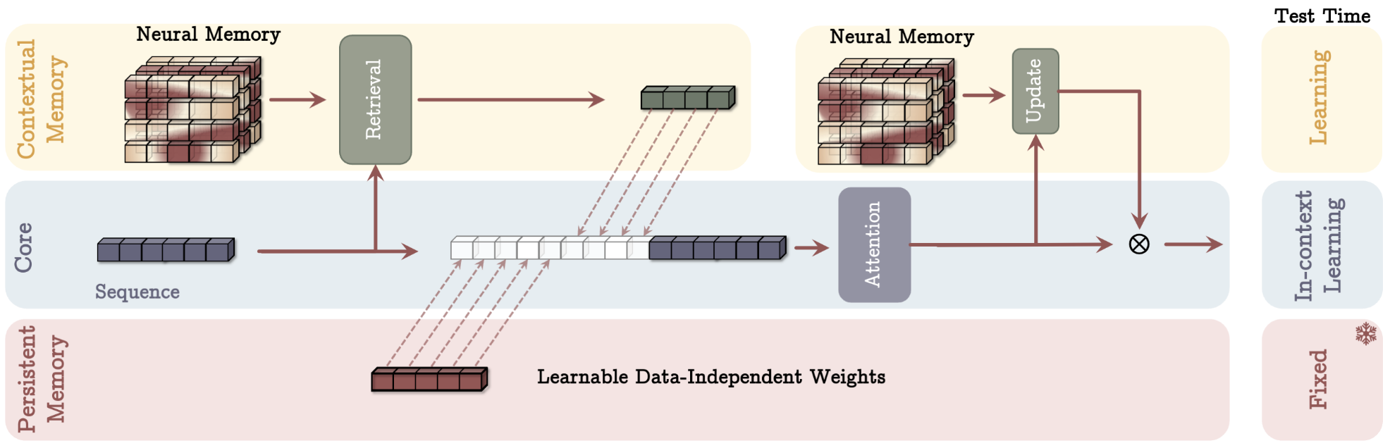
- MAC — Memory as Context:
Retrieve memory → concatenate with persistent memory → feed into attention → Best long-context performance.
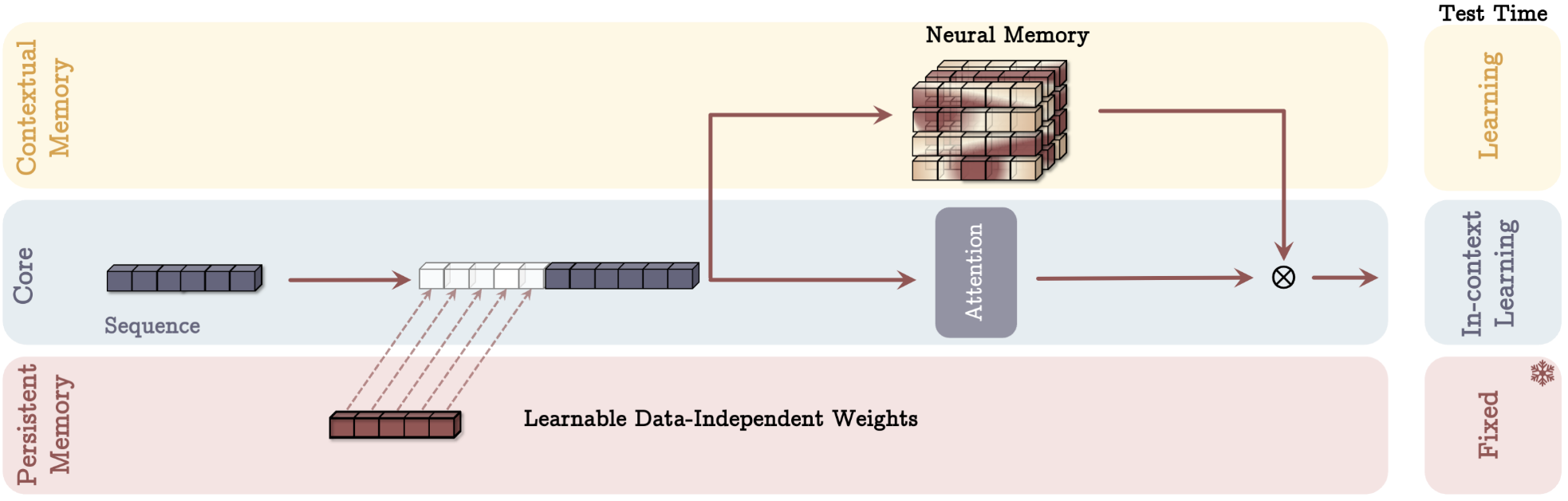
- MAG — Memory as Gate: Combine Sliding Window Attention output and memory output via gating.
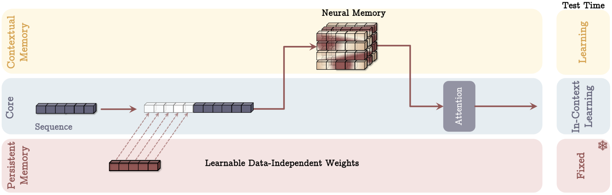
- MAL — Memory as Layer: Sequential: LMM → Sliding Window Attention. Simpler but weaker performance.
3. Novelty
3.1. Memory Structure
- Titans introduce a long-term memory (LMM) that can learn and store information across millions of tokens.
- This memory is a deep, learnable module, not just a matrix or KV-cache.
- Three designs (MAL) show flexible ways to combine long-term memory with short-term attention.
3.2. Memory Update
- LMM learns during inference, using a simple idea: more surprising tokens are written more strongly.
- Updates use momentum (past surprise + current surprise) for stability.
- A forget gate decides how much old memory to remove to avoid overflow.
3.3. Memory Retrieval
- LMM learns a key → value mapping, acting like a smart, compressing KV-cache.
- The model retrieves long-term information when needed and mixes it with short-term attention (SWA).
4. More Details
4.1. What is M?
M is a learnable function (an MLP) that stores long-term information.
$$ M : R^d \rightarrow R^d $$
It takes a vector (key or query) and outputs another vector (a “memory value”).
You can think of M as a neural dictionary:
- input = address
- output = content
Except this dictionary learns at test time, and compresses many past tokens into a fixed-sized neural network.
4.2. What does M do during RETRIEVAL?
Retrieval input: query
$$ q_t = x_t W_Q $$
Memory returns:
$$ y^{(LMM)}_t = M(q_t) $$
Meaning:
“Given this query, what long-term knowledge have we stored that matches it?”
So during retrieval:
- M behaves as a lookup function
- q = the question
- M(q) = the answer from long-term memory
Here, all the knowledge is compressed inside the MLP weights.
4.3. What does M do during UPDATE?
Update input: key
$$ k_t = x_t W_K,\qquad v_t = x_t W_V $$
Memory tries to learn the mapping:
$$ M(k_t) \approx v_t $$
Error:
$$ \ell = | M(k_t) - v_t |^2 $$
Gradient:
$$ g_t = \nabla_{M} \ell $$
Memory update:
$$ M \leftarrow M - \theta g_t $$
Meaning:
“Given this key, the correct value should be v. Update yourself so you can remember this in the future.”
So during update:
- M behaves as a learnable associative memory
- k = the address
- v = the content
- M learns: k → v
This is exactly like writing to a KV-cache — except the cache is a learnable neural network that can compress, forget, and generalize.
4.4. What role does M play?
Role 1: long-term storage
M learns from (k,v) pairs:
$$ M(k) \approx v $$
This is how it stores information.
Role 2: long-term retrieval
M responds to queries:
$$ M(q) = \text{long-term memory output} $$
This is how it retrieves information.
Why both? Because:
- Keys write into memory
- Queries read from memory
- Both must use the same space so they match