1. Introduction
Modern sequence models (especially Transformers) achieve strong performance due to their ability to learn from long contexts at scale. However, Transformers suffer from quadratic complexity and linearly growing memory (KV cache), which limits long-context modeling. To overcome this, recent research develops efficient recurrent alternatives that compress information into fixed-size memory, focusing on:
- Learning rules (from Hebbian → Delta → new variants)
- Forget gates (from LSTM → Mamba → Titan gates)
- Memory architectures (vector memory in RetNet, LRU; deep memory in Titans and TTT)
These advances raise a central question:
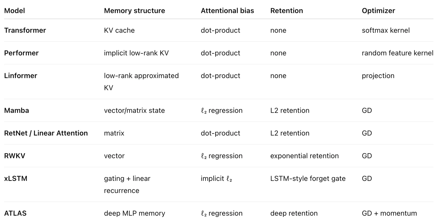
The authors reinterpret Transformers, Titans, and modern linear RNNs as associative memory systems, guided by a new concept called attentional bias—the internal objective that determines how models learn mappings between keys and values. Surprisingly, they observe that almost all existing models use only two types of attentional bias: dot-product similarity or ℓ₂ regression.
Based on this insight, they reinterpret forgetting mechanisms as retention ℓ₂-regularization, then introduce Miras, a general design framework defined by four choices:
- Attentional bias (memory objective)
- Retention gate
- Memory architecture
- Memory learning algorithm (optimizer)
Using Miras, they create three new sequence models—Moneta, Yaad, and Memora—that incorporate new attentional biases and robust forgetting mechanisms. Experiments show that these models outperform current architectures in language modeling, reasoning, and memory-intensive tasks.
2. Method
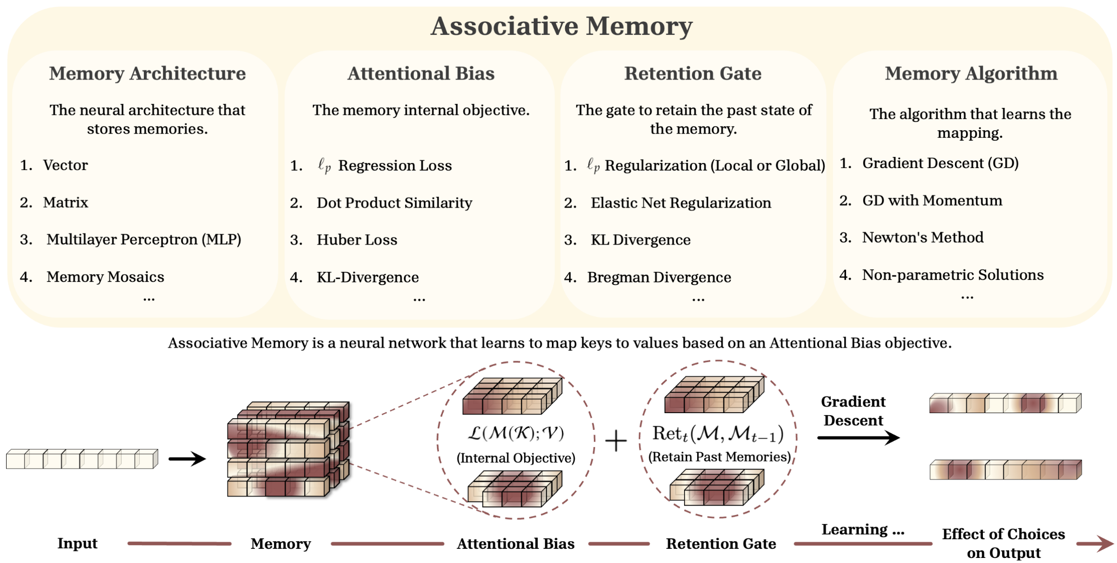
2.1. Associative Memory and Attentional Bias
Associative memory maps keys (K) to values (V). The mapping is learned by optimizing an objective $\mathcal{L}$ called attentional bias.
Formally, memory $\mathcal{M}$ is learned by:
$$ \mathcal{M}^* = \arg\min_{\mathcal{M}} \mathcal{L}(\mathcal{M}(K); V). $$
Remark 1
- When memory is parameterized by a matrix $W$, we optimize $W$, not $\mathcal{M}$.
- We may also add regularization $R(W)$ to retain past memory.
Remark 2
- Learning keys–values is a meta-learning problem: inner-loop optimizes memory; outer-loop optimizes the rest of the network.
Remark 3
- Forgetting is not explicit erasing; rather, the model may fail to retrieve past memory.
- Therefore they use the term “Retention Gate”, not “Forget Gate”.
Remark 4
- Most modern sequence models optimize the associative memory objective (attentional bias) via gradient descent.
- The theory applies beyond GD, any optimization method can be used.
2.1.1. Learning to Memorize and Retain (Optimization View)
Memory is updated by gradient descent:
$$ W_t = W_{t-1} - \eta_t \nabla \ell(W_{t-1}; k_t, v_t), $$
where $\ell$ is the attentional bias applied to the latest pair.
2.1.2. Viewpoint 1: Online Regression and Follow-The-Regularized-Leader
Gradient descent can be interpreted as minimizing a sequence of losses:
$$ \ell(W; k_1, v_1), \ell(W; k_2, v_2), \ldots $$
Equivalent formulation:
$$ W_t = \arg\min_W \sum_{i=1}^t \langle W - W_{t-1}, \nabla \ell(W_{t-1}; k_i, v_i) \rangle + \frac{1}{2\eta_t}|W|^2. $$
The first term measures how well memory fits new data;
the second term is a regularizer that stabilizes memory size.
General FTRL form:
$$ W_t = \arg\min_{W \in \mathcal{W}} \left(\sum_{i=1}^t \tilde{\ell}_i(W; k_i, v_i)\right) + \frac{1}{\eta_t} R_t(W). $$
Here:
- $\tilde{\ell}_i$ = approximated attentional bias
- $R_t(W)$ = memory stability regularizer
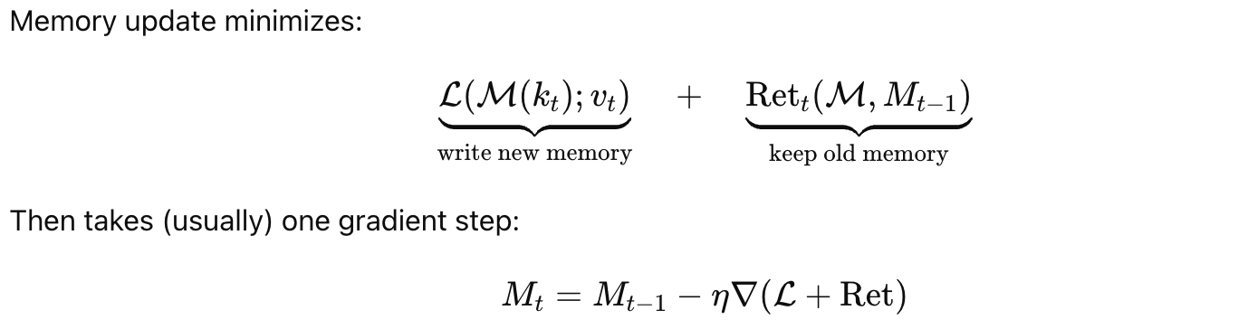
2.1.3. Viewpoint 2: Learning the Latest Token While Retaining Previous Memory
Another interpretation decomposes memory update into: Learning new info + Retaining old memory.
Equivalent update:
$$ W_t = \arg\min_W \Big( \langle W - W_{t-1}, \nabla \ell(W_{t-1}; k_t, v_t)\rangle + \frac{1}{2\eta_t} |W - W_{t-1}|^2 \Big). $$
The form generalizes to:
$$ W_t = \arg\min_{W \in \mathcal{W}} \Big( \tilde{\ell}_t(W; k_t, v_t) + \text{Ret}_t(W, W{t-1}) \Big). $$
- Attentional Bias: $\tilde{\ell}_t(W; k_t, v_t)$ → learns new key–value mapping.
- Retention: $\text{Ret}_t(W, W{t-1})$ → encourages memory to stay close to its previous state.
Retention has local and global components:
$$ \text{Ret}t(W, W{t-1}) = \frac{1}{\eta_t} D_t(W, W_{t-1}) + \frac{1}{\alpha_t} G_t(W). $$
- $D_t$: local retention → prevents forgetting
- $G_t$: global retention → controls memory magnitude
2.1.4. Connection Between the Two Viewpoints
Both viewpoints describe the same process using online optimization concepts. The two formulations are equivalent under mild assumptions.
- The FTRL viewpoint emphasizes loss over time + regularization.
- The Learning–Retaining viewpoint emphasizes new learning + memory retention.
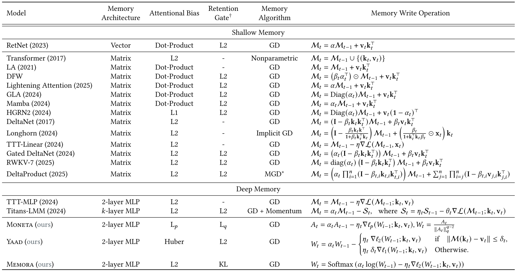
2.2. MIRAS
MIRAS says every sequence model is defined by 4 choices:
Memory Structure
What the memory looks like vector, matrix, MLP.
Attentional Bias
The loss used to learn key→value mapping like dot-product, $\ell_2$, $\ell_p$, Huber, KL. → loss function
Retention Gate
Controls how much old memory is kept. Like: $|W - W_{t-1}|^2$, KL divergence, elastic net, etc.
Memory Algorithm
How memory is updated (GD, momentum, Newton, etc.). → optimizer
All existing models fit this form.
Examples:
- Hebbian RNNs (RetNet, LA)
$$ M_t = \alpha M_{t-1} + v_t k_t^\top $$
Delta rule models (DeltaNet, RWKV)
They optimize MSE: $|M(k_t) - v_t|^2$.
Titans / TTT
Use deep memory + gradient descent with retention.
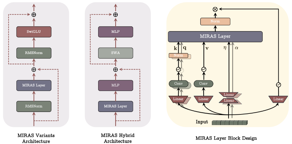
2.3. Architecture Backbone and Fast Training
Architectural Backbone for Miras’s Variants: Moneta, Yaad, and Memora
- Replace the attention block with a MIRAS block inside a Llama-style model.
- Use modern components: SwiGLU MLPs, RoPE, RMSNorm, depthwise conv, and ℓ₂-normed q/k.
Channel-wise Parameters
- Parameters like $\eta_t, \delta_t, \alpha_t$ are learned per channel.
- To reduce cost, apply low-rank projections.
Hybrid Models
- MIRAS layers can be combined with Sliding Window Attention (SWA).
Parallel Training
- Recurrence is broken using chunking: split the sequence into chunks and compute gradients per chunk.
- This makes training fast and parallelizable.
Core recurrence idea
Inside a chunk, replace:
$$ M_t = \alpha_t M_{t-1} - \eta_t \nabla \ell $$
with a parallel form:
$$ M_t = \beta_t M_0 - \sum_{i=1}^t \frac{\beta_t}{\beta_i}\eta_i\nabla\ell(M_0;k_i,v_i) $$
so no step-by-step recurrence is needed.
3. Comparison