1. Problems
1.1. Multimodal action distributions
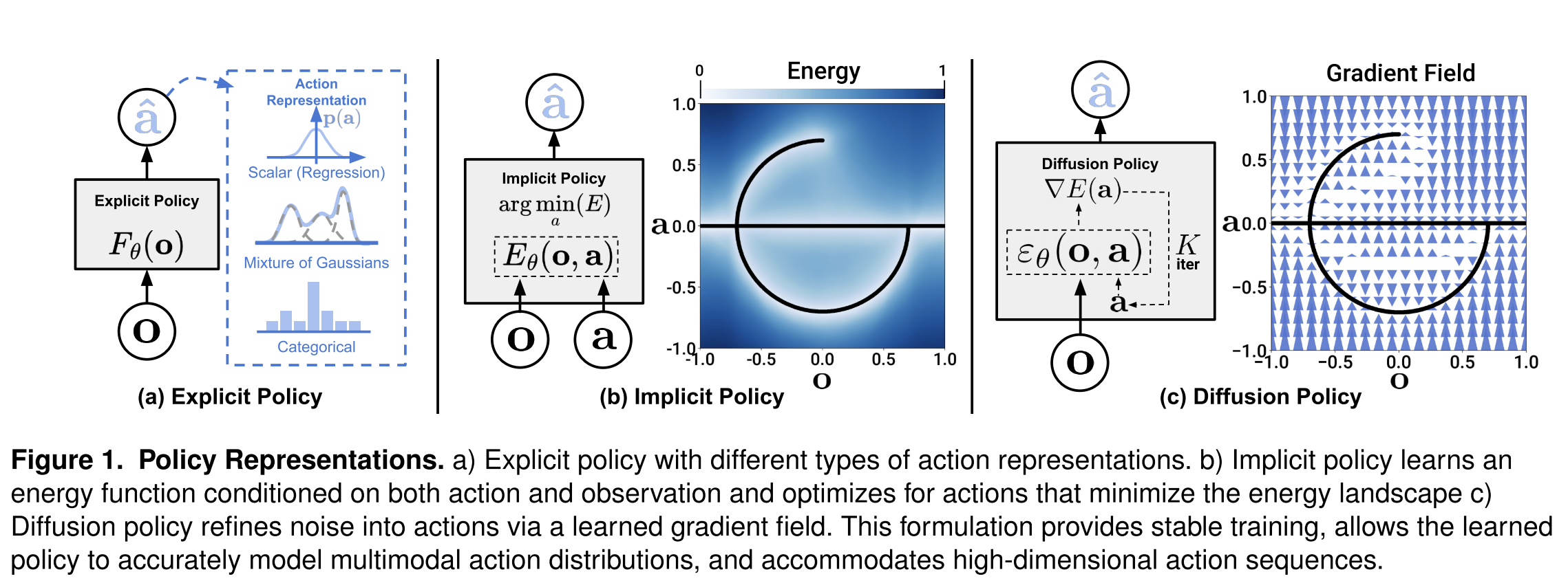
In demonstrations, the same visual/state observation can reasonably lead to different next actions (e.g., go left vs right around an obstacle, different grasp styles, different sub-goal order). Explicit regressions (single Gaussian / MSE) tend to average modes and become “invalid” actions.
1.2. High-dimensional output and temporal consistency
Robot control is sequential. Predicting one step at a time often produces tiny or mode-switching (action at t chooses mode A, action at t+1 chooses mode B). But predicting a whole action sequence is high-dimensional and hard for many policy classes.
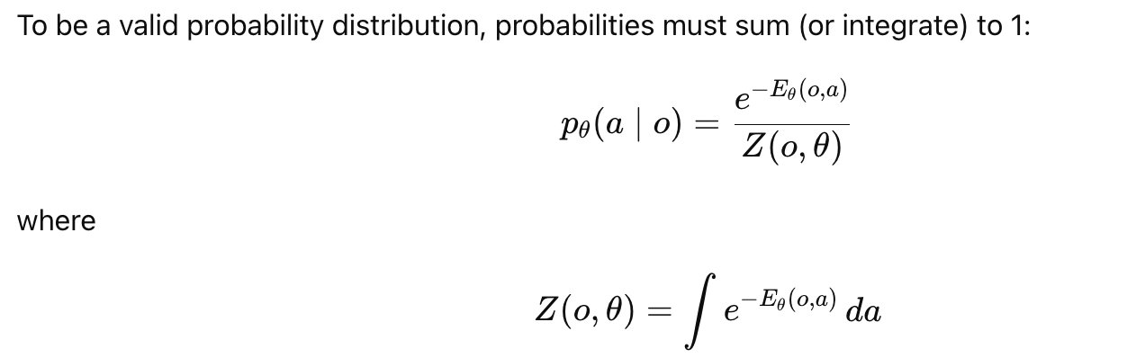
1.3. Training instability of implicit / energy-based policies (IBC)
Implicit policies (IBC) represent $p(a|o)\propto e^{-E(o,a)}$ but training needs negative samples to estimate the intractable normalization $Z(o,\theta)$, which can be inaccurate and causes instability and checkpoint sensitivity.
1.4. Real-world deployment constraints
Policies must be fast enough for closed-loop control; naïve diffusion conditioning on both state and action trajectories can be expensive.
2. Method
Instead of outputting an action directly, the policy outputs a denoising direction field over actions and iteratively refines noise into an action sequence.
2.1. DDPM sampling view:
Start from Gaussian noise $x^K$. For $k=K\to1$, update (x → x - predicted noise + noise):
$$ x^{k-1}=\alpha\Big(x^k-\gamma,\varepsilon_\theta(x^k,k)+\mathcal N(0,\sigma^2 I)\Big) $$
where $\varepsilon_\theta$ is a learned “noise predictor” (can be seen as a learned gradient field).
2.2. Adapt DDPM to visuomotor policy:
The denoising update becomes:
$$ A_t^{k-1}=\alpha\Big(A_t^k-\gamma,\varepsilon_\theta(O_t, A_t^k, k)+\mathcal N(0,\sigma^2 I)\Big) $$
So the network input is (observation features, noisy action sequence, diffusion step k) and output is predicted noise / denoising direction for that step.
2.3. Training:
Pick a clean expert action sequence $A_t^0$, sample a diffusion step $k$, add noise $\varepsilon_k$, train (actual noise added to the expert actions = predicted noise):
$$ L=\mathrm{MSE}\big(\varepsilon_k,\ \varepsilon_\theta(O_t,\ A_t^0+\varepsilon_k,\ k)\big) $$
This avoids EBM’s intractable $Z(o,\theta)$ and negative sampling.
2.4. Key technical contributions to make it work well on robots
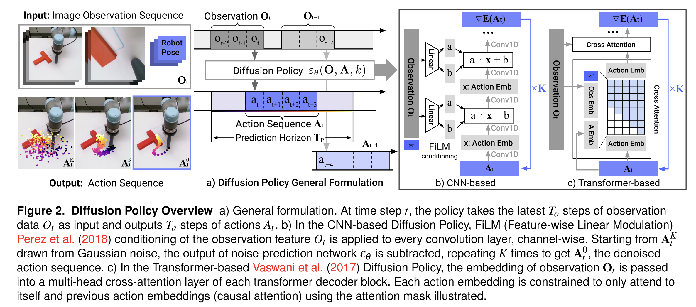
Closed-loop action sequences + receding horizon control
At time $t$, use last $T_o$ observations $O_t$ to predict a future horizon of actions $T_p$, execute only $T_a$ steps, then re-plan (receding horizon). Warm-start the next plan for smoothness.
Visual conditioning for speed
Treat vision as conditioning: compute visual features once and reuse them across diffusion iterations, enabling real-time inference.
Time-series diffusion transformer
A transformer-based denoiser improves tasks requiring high-frequency action changes / velocity control, reducing over-smoothing seen in CNN temporal models.
- The expert trajectory contains: move → stop → move quickly → stop
- A CNN tends to produce: move → slow → slow → slow
Real-time acceleration via DDIM
Use DDIM(Denoising Diffusion Implicit Models) to reduce latency (reported ~0.1s on RTX 3080 for real-world). Train with many diffusion steps (e.g., 100), but infer with fewer (e.g., 10–16)
3. Novelty
3.1. New policy representation: “diffusion on action space”
They frame a visuomotor policy as a conditional denoising diffusion process over action sequences, not direct regression (explicit) and not energy-minimization with negatives (EBM).
3.2. Handles multimodality naturally via stochastic sampling + iterative refinement
Different random initializations $A_t^K$ and stochastic updates let the policy represent and sample multiple valid action modes, and action-sequence prediction helps it commit to one mode per rollout.
3.3. Scales to high-dimensional outputs by predicting action sequences
Diffusion models are known to work in high dimension; they exploit this to model whole trajectories, improving temporal consistency and robustness (including idle-action segments).
3.4. Training stability advantage over IBC/EBM
They explicitly explain stability: EBM needs $Z(o,\theta)$ and negative sampling; diffusion learns the score $\nabla_a \log p(a|o)$ which does not depend on $Z$, so training/inference avoid that source of instability.
3.5. System-level robotics contributions
Receding-horizon execution, efficient visual conditioning(Extract observations once, then reuse them across all diffusion steps), and a time-series diffusion transformer are concrete robotics-driven changes that “unlock” diffusion for real-world visuomotor control.